Section:
New Results
Application of shape and topology design to biology and medicine
Assessing the ability of the 2D Fisher-KPP equation to model cell-sheet wound closure
Participants :
Abderrahmane Habbal, Hélène Barelli [Univ. Nice Sophia Antipolis, CNRS, IPMC] , Grégoire Malandain [Inria, EPI Morpheme] .
We address in this joint collaboration the ability of the widely used Fisher-KPP equations to render some of the dynamical features of epithelial cell-sheets during wound closure.
Our approach is based on nonlinear parameter identification, in a two-dimensional setting, and using advanced 2D image processing of the video acquired sequences. As original contribution, we lead a detailed study of the profiles of the classically used cost functions, and we address the "wound constant speed" assumption, showing that it should be handled with care.
We study five MDCK cell monolayer assays in a reference, activated and inhibited migration conditions. Modulo the inherent variability of biological assays, we show that in the assay where migration is not exogeneously activated or inhibited, the wound velocity is constant. The Fisher-KPP equation is able to accurately predict, until the final closure of the wound, the evolution of the wound area, the mean velocity of the cell front, and the time at which the closure occurred.
We also show that for activated as well as for inhibited migration assays, many of the cell-sheet dynamics cannot be well captured by the Fisher-KPP model. Original unexplored utilizations of the model such as wound assays classification based on the calibrated diffusion and proliferation rate parameters is ongoing.[49] [76]
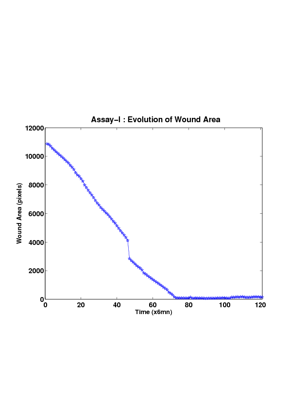
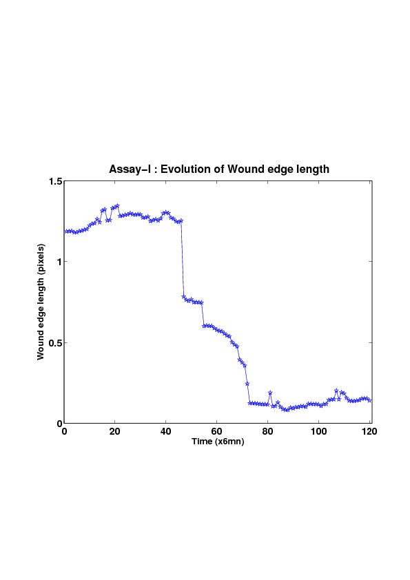
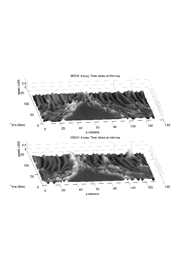
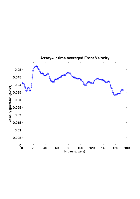
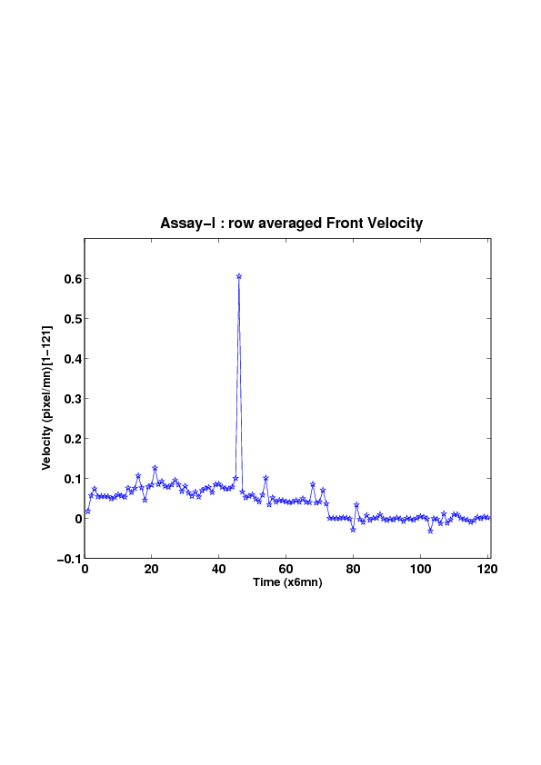
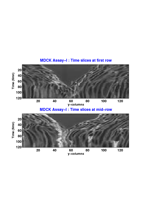
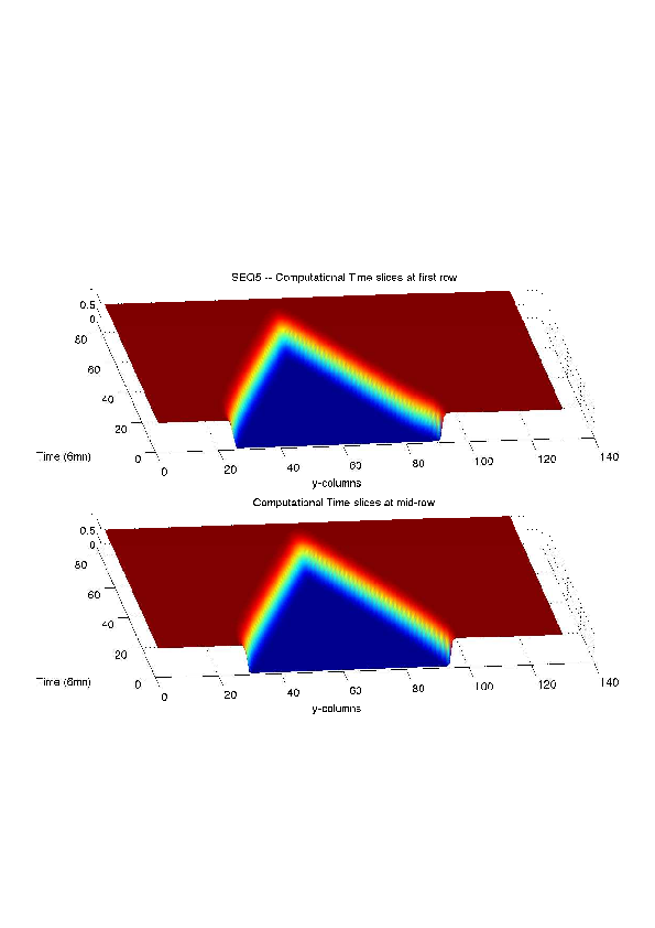
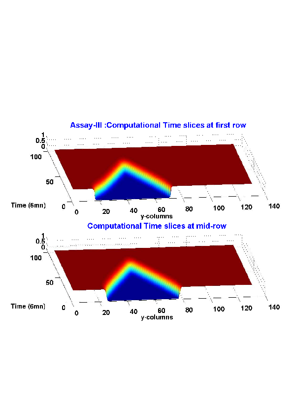
Figure
5. A regular wound assay (a) Time evolution of wound area (in pixel). (b) Time evolution of the leading-edge length (in pixel). (c) 3D view at first and mid-rows. (d) Mean (in time) velocity of pixels located at the leading edge (in pixel/min). (e) Averaged (in space) leading-edge velocity (in pixel/min). (f) 2D view at first and mid-rows.
|
|
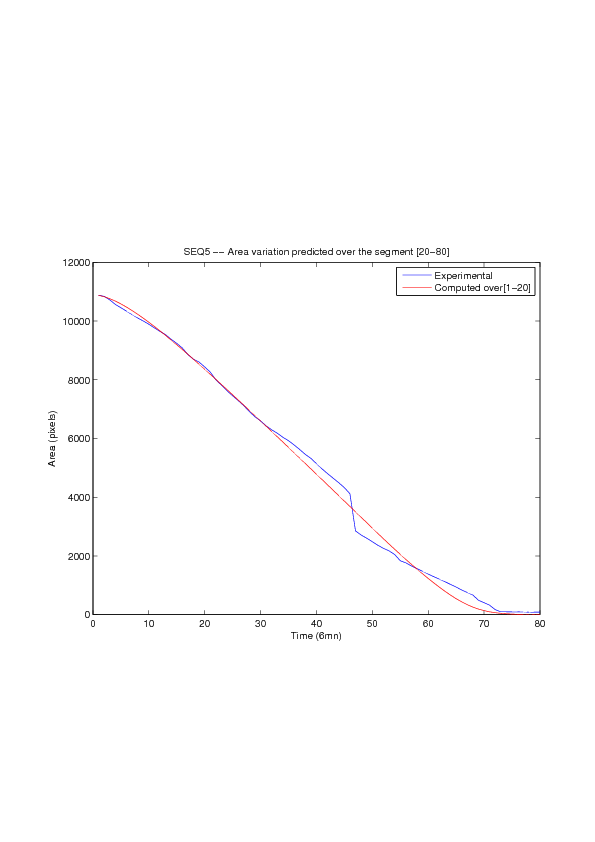
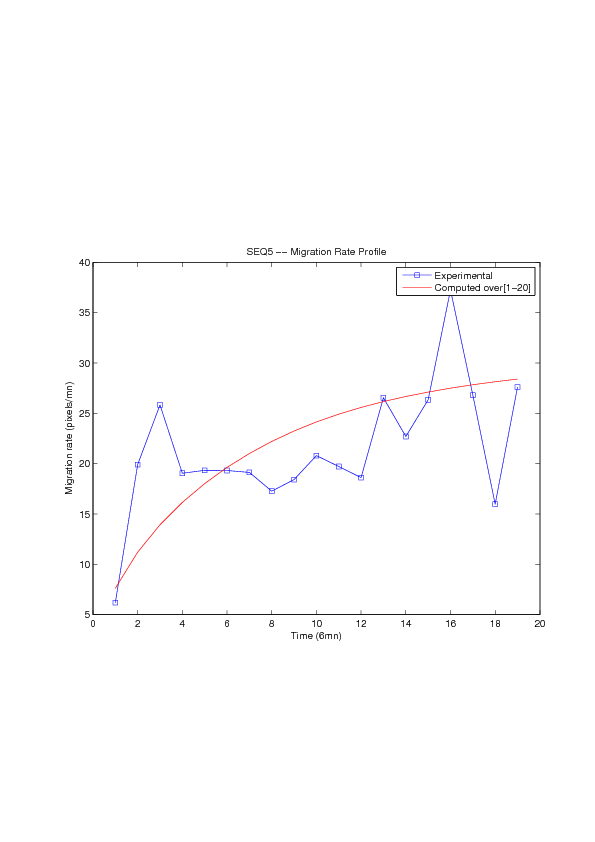
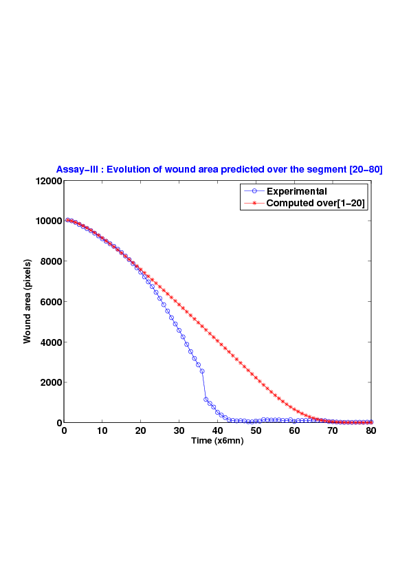
Figure
6. A regular wound assay. Computational vs experimental wound evolution. (a) Time variation of experimental (blue) versus computed (red) wound area (in pixel). (b) Time variation of the experimental (blue-dot) versus computed (red) migration rate (in pixel/min). (c) 3D view at first and mid-rows.
|
|
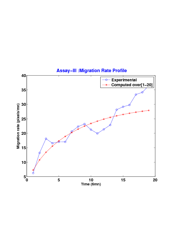
Figure
7. An accelerating activated wound assay. Computational vs experimental wound evolution. (a) Time variation of experimental (blue) versus computed (red) wound area (in pixel). (b) Time variation of the experimental (blue-dot) versus computed (red) migration rate (in pixel/min). (c) 3D view at first and mid-rows.
|
|