<?xml version="1.0" encoding="utf-8"?>
<!DOCTYPE html PUBLIC "-//W3C//DTD XHTML 1.1 plus MathML 2.0 plus SVG 1.1//EN" "http://www.w3.org/2002/04/xhtml-math-svg/xhtml-math-svg.dtd">
<html xmlns="http://www.w3.org/1999/xhtml">
  <head>
    <meta http-equiv="Content-Type" content="application/xhtml+xml; charset=utf-8"/>
    <title>Project-Team:APICS</title>
    <link rel="stylesheet" href="../static/css/raweb.css" type="text/css"/>
    <meta name="description" content="New Results - Source recovery problems"/>
    <meta name="dc.title" content="New Results - Source recovery problems"/>
    <meta name="dc.creator" content="Laurent Baratchart"/>
    <meta name="dc.creator" content="Sylvain Chevillard"/>
    <meta name="dc.creator" content="Juliette Leblond"/>
    <meta name="dc.creator" content="Christos Papageorgakis"/>
    <meta name="dc.creator" content="Olga Permiakova"/>
    <meta name="dc.creator" content="Dmitry Ponomarev"/>
    <meta name="dc.subject" content=""/>
    <meta name="dc.publisher" content="INRIA"/>
    <meta name="dc.date" content="(SCHEME=ISO8601) 2014-01"/>
    <meta name="dc.type" content="Report"/>
    <meta name="dc.language" content="(SCHEME=ISO639-1) en"/>
    <meta name="projet" content="APICS"/>
    <!-- Piwik -->
    <script type="text/javascript" src="/rapportsactivite/piwik.js"></script>
    <noscript><p><img src="//piwik.inria.fr/piwik.php?idsite=49" style="border:0;" alt="" /></p></noscript>
    <!-- End Piwik Code -->
  </head>
  <body>
    <div class="tdmdiv">
      <div class="logo">
        <a href="http://www.inria.fr">
          <img style="align:bottom; border:none" src="../static/img/icons/logo_INRIA-coul.jpg" alt="Inria"/>
        </a>
      </div>
      <div class="TdmEntry">
        <div class="tdmentete">
          <a href="uid0.html">Project-Team Apics</a>
        </div>
        <span>
          <a href="uid1.html">Members</a>
        </span>
      </div>
      <div class="TdmEntry">Overall Objectives<ul><li><a href="./uid3.html">Research Themes</a></li></ul></div>
      <div class="TdmEntry">Research Program<ul><li><a href="uid7.html&#10;&#9;&#9;  ">Introduction</a></li><li><a href="uid11.html&#10;&#9;&#9;  ">Range of inverse problems</a></li><li><a href="uid17.html&#10;&#9;&#9;  ">Approximation</a></li></ul></div>
      <div class="TdmEntry">Application Domains<ul><li><a href="uid25.html&#10;&#9;&#9;  ">Introduction</a></li><li><a href="uid26.html&#10;&#9;&#9;  ">Inverse source problems in EEG</a></li><li><a href="uid27.html&#10;&#9;&#9;  ">Inverse magnetization problems</a></li><li><a href="uid29.html&#10;&#9;&#9;  ">Free boundary problems</a></li><li><a href="uid30.html&#10;&#9;&#9;  ">Identification and design of microwave devices</a></li></ul></div>
      <div class="TdmEntry">New Software and Platforms<ul><li><a href="uid39.html&#10;&#9;&#9;  ">
        RARL2
      </a></li><li><a href="uid43.html&#10;&#9;&#9;  ">RGC</a></li><li><a href="uid44.html&#10;&#9;&#9;  ">
        PRESTO-HF
      </a></li><li><a href="uid49.html&#10;&#9;&#9;  ">
        Dedale-HF
      </a></li><li><a href="uid51.html&#10;&#9;&#9;  ">
        easyFF
      </a></li><li><a href="uid52.html&#10;&#9;&#9;  ">
        FindSources3D
      </a></li><li><a href="uid56.html&#10;&#9;&#9;  ">
        Sollya
      </a></li></ul></div>
      <div class="TdmEntry">New Results<ul><li class="tdmActPage"><a href="uid58.html&#10;&#9;&#9;  ">Source recovery problems</a></li><li><a href="uid63.html&#10;&#9;&#9;  ">Boundary value problems</a></li><li><a href="uid64.html&#10;&#9;&#9;  ">Matching problems and their applications - De-embedding of filters in multiplexers</a></li><li><a href="uid71.html&#10;&#9;&#9;  ">Stability of amplifiers</a></li><li><a href="uid76.html&#10;&#9;&#9;  ">Approximation</a></li></ul></div>
      <div class="TdmEntry">Bilateral Contracts and Grants with Industry<ul><li><a href="uid80.html&#10;&#9;&#9;  ">Contract CNES-Inria-XLIM</a></li><li><a href="uid81.html&#10;&#9;&#9;  ">Contract CNES-Inria-UPV/EHU</a></li><li><a href="uid82.html&#10;&#9;&#9;  ">Contract BESA GmbH-Inria</a></li></ul></div>
      <div class="TdmEntry">Partnerships and Cooperations<ul><li><a href="uid85.html&#10;&#9;&#9;  ">Regional Initiatives</a></li><li><a href="uid87.html&#10;&#9;&#9;  ">National Initiatives</a></li><li><a href="uid90.html&#10;&#9;&#9;  ">European Initiatives</a></li><li><a href="uid94.html&#10;&#9;&#9;  ">International Initiatives</a></li><li><a href="uid106.html&#10;&#9;&#9;  ">International Research Visitors</a></li><li><a href="uid117.html&#10;&#9;&#9;  ">List of international and industrial partners</a></li></ul></div>
      <div class="TdmEntry">Dissemination<ul><li><a href="uid122.html&#10;&#9;&#9;  ">Promoting Scientific Activities</a></li><li><a href="uid137.html&#10;&#9;&#9;  ">Teaching - Supervision - Juries</a></li><li><a href="uid148.html&#10;&#9;&#9;  ">Popularization</a></li><li><a href="uid152.html&#10;&#9;&#9;  ">Community services</a></li></ul></div>
      <div class="TdmEntry">
        <div>Bibliography</div>
      </div>
      <div class="TdmEntry">
        <ul>
          <li>
            <a id="tdmbibentmajor" href="bibliography.html">Major publications</a>
          </li>
          <li>
            <a id="tdmbibentyear" href="bibliography.html#year">Publications of the year</a>
          </li>
          <li>
            <a id="tdmbibentfoot" href="bibliography.html#References">References in notes</a>
          </li>
        </ul>
      </div>
    </div>
    <div id="main">
      <div class="mainentete">
        <div id="head_agauche">
          <small><a href="http://www.inria.fr">
	    
	    Inria
	  </a> | <a href="../index.html">
	    
	    Raweb 
	    2014</a> | <a href="http://www.inria.fr/en/teams/apics">Presentation of the Project-Team APICS</a> | <a href="http://team.inria.fr/apics/">APICS Web Site
	  </a></small>
        </div>
        <div id="head_adroite">
          <table class="qrcode">
            <tr>
              <td>
                <a href="apics.xml">
                  <img style="align:bottom; border:none" alt="XML" src="../static/img/icons/xml_motif.png"/>
                </a>
              </td>
              <td>
                <a href="apics.pdf">
                  <img style="align:bottom; border:none" alt="PDF" src="IMG/qrcode-apics-pdf.png"/>
                </a>
              </td>
              <td>
                <a href="../apics/apics.epub">
                  <img style="align:bottom; border:none" alt="e-pub" src="IMG/qrcode-apics-epub.png"/>
                </a>
              </td>
            </tr>
            <tr>
              <td/>
              <td>PDF
</td>
              <td>e-Pub
</td>
            </tr>
          </table>
        </div>
      </div>
      <!--FIN du corps du module-->
      <br/>
      <div class="bottomNavigation">
        <div class="tail_aucentre">
          <a href="./uid56.html" accesskey="P"><img style="align:bottom; border:none" alt="previous" src="../static/img/icons/previous_motif.jpg"/> Previous | </a>
          <a href="./uid0.html" accesskey="U"><img style="align:bottom; border:none" alt="up" src="../static/img/icons/up_motif.jpg"/>  Home</a>
          <a href="./uid63.html" accesskey="N"> | Next <img style="align:bottom; border:none" alt="next" src="../static/img/icons/next_motif.jpg"/></a>
        </div>
        <br/>
      </div>
      <div id="textepage">
        <!--DEBUT2 du corps du module-->
        <h2>Section: 
      New Results</h2>
        <h3 class="titre3">Source recovery problems</h3>
        <p class="participants"><span class="part">Participants</span> :
	Laurent Baratchart, Sylvain Chevillard, Juliette Leblond, Christos Papageorgakis, Olga Permiakova, Dmitry Ponomarev.</p>
        <p>The research in this section is partly joint work with Qian Tao (Univ. Macao).</p>
        <p>It was proved in <a href="./bibliography.html#apics-2014-bid18">[38]</a> 
that a vector field with <span class="math"><math xmlns="http://www.w3.org/1998/Math/MathML"><mrow><mi>n</mi><mo>+</mo><mn>1</mn></mrow></math></span> components on <span class="math"><math xmlns="http://www.w3.org/1998/Math/MathML"><msup><mrow><mi>ℝ</mi></mrow><mi>n</mi></msup></math></span>
can be expressed uniquely as the sum of (the trace on <span class="math"><math xmlns="http://www.w3.org/1998/Math/MathML"><msup><mrow><mi>ℝ</mi></mrow><mi>n</mi></msup></math></span> of) a
harmonic gradient in the upper half-space,
of (the trace on <span class="math"><math xmlns="http://www.w3.org/1998/Math/MathML"><msup><mrow><mi>ℝ</mi></mrow><mi>n</mi></msup></math></span> of) a
harmonic gradient in the lower half-space,
and of a tangential divergence free vector field on <span class="math"><math xmlns="http://www.w3.org/1998/Math/MathML"><msup><mrow><mi>ℝ</mi></mrow><mi>n</mi></msup></math></span>.
This decomposition, that we call the <i>Hardy-Hodge</i> decomposition,
is valid not only for <span class="math"><math xmlns="http://www.w3.org/1998/Math/MathML"><msup><mi>L</mi><mi>p</mi></msup></math></span> vector fields as mentioned in
Section <a title="Approximation" href="./uid17.html#uid18">
	3.3.1</a> , but in much more general distribution spaces
like <span class="math"><math xmlns="http://www.w3.org/1998/Math/MathML"><msup><mi>W</mi><mrow><mo>-</mo><mi>∞</mi><mo>,</mo><mi>p</mi></mrow></msup></math></span> which contains all distributions with compact support
or <span class="math"><math xmlns="http://www.w3.org/1998/Math/MathML"><mrow><mi>B</mi><mi>M</mi><msup><mi>O</mi><mrow><mo>-</mo><mi>∞</mi></mrow></msup></mrow></math></span> which contains all finite sums of derivatives of bounded
functions. This year we extended the decomposition to smooth hypersurfaces,
where divergence-free distributions may be defined as those annihilating
tangential gradient vector fields. We also studied the case where the
hypersurface is only Lipschitz smooth, and then we proved the
decomposition in <span class="math"><math xmlns="http://www.w3.org/1998/Math/MathML"><msup><mi>L</mi><mi>p</mi></msup></math></span> provided that <span class="math"><math xmlns="http://www.w3.org/1998/Math/MathML"><mi>p</mi></math></span> is close enough to 2
(how close depends on the Lipschitz constant of the hypersurface).</p>
        <p>The Hardy-Hodge decomposition was used in <a href="./bibliography.html#apics-2014-bid18">[38]</a> 
to find the kernel of the planar magnetization operator, namely a
potential of
the form (<a title="Inverse magnetization problems" href="./uid27.html#uid28">1</a> ) with <span class="math"><math xmlns="http://www.w3.org/1998/Math/MathML"><mi>m</mi></math></span> supported in a plane generates the zero
field above that plane if, and only if there is no harmonic
gradient from below in the Hardy-Hodge decomposition of <span class="math"><math xmlns="http://www.w3.org/1998/Math/MathML"><mi>m</mi></math></span>.
The above mentioned generalization is now to the effect that a magnetization
supported on a bounded
closed surface (<i>e.g.</i> a sphere)
is silent in the unbounded component of
the complement of that surface if, and only if there is no harmonic
gradient from inside in its Hardy-Hodge decomposition.
An article is being written on this topic.</p>
        <p>We also considered the case where <span class="math"><math xmlns="http://www.w3.org/1998/Math/MathML"><mi>m</mi></math></span> is compactly supported in the
bounded component of the complement of that surface. Then <span class="math"><math xmlns="http://www.w3.org/1998/Math/MathML"><mi>m</mi></math></span> is silent if
and only if it is the sum of a divergence-free distribution and of finitely
many derivatives of gradients of Sobolev functions
having zero trace on the surface <a href="./bibliography.html#apics-2014-bid67">[41]</a> .</p>
        <p>These results shed light on the indeterminacy of inverse source problems.</p>
        <a name="uid59"/>
        <h4 class="titre4">EEG</h4>
        <p>This work is conducted in collaboration with Maureen Clerc and Théo
Papadopoulo from the Athena EPI, and with Jean-Paul Marmorat (Centre de mathématiques appliquées - CMA, École des Mines de Paris).</p>
        <p>In 3-D, functional or clinically active regions
in the cortex are often modeled by point-wise sources that must be
localized from measurements of a potential on the scalp. Inside the cortex,
identified to a ball after the cortical mapping step,
the potential satisfies a Poisson equation whose right-hand side is a linear
combination of gradients of Dirac masses (the sources in EEG).
In the work <a href="./bibliography.html#apics-2014-bid23">[3]</a>  it was shown how
best rational approximation on a family of
circles, cut along parallel planes on the sphere, can
be used to recover the sources when they are at most 2 of them.
Later, results on the behavior of poles in
best rational approximation of fixed degree to functions with branch points
<a href="./bibliography.html#apics-2014-bid21">[6]</a>  helped justifying the technique for
finitely many sources (see section <a title="Inverse source problems in EEG" href="./uid26.html">
	4.2</a> ).</p>
        <p>The dedicated software FindSources3D (see section <a title="&#10;        FindSources3D&#10;      " href="./uid52.html">
	5.6</a> ),
developed, in collaboration with the team Athena and the CMA,
dwells on these ideas. Functions to be approximated in 2-D slices
turn out to have additional <i>multiple</i> poles at their branch points
so that, in the rational approximation step,
it is beneficial to consider approximants with
multiple poles as well
(for EEG data, one should consider <i>triple</i> poles). Though numerically
observed in <a href="./bibliography.html#apics-2014-bid24">[9]</a> , there is no mathematical
justification so far why these multiple poles are attracted more strongly than
simple poles to the singularities of the approximated function.
This intriguing property, however,
definitely helps source recovery <a href="./bibliography.html#apics-2014-bid66">[28]</a> . This year we used it to automatically estimate the “most plausible”
number of sources (numerically: up to 3 at the moment).
Such enhancements were prompted by
a developing collaboration with the BESA company,
which is interested in automatic detection of the number of sources
(which was left to the user until recently).</p>
        <p>Soon, magnetic data from MEG (magneto-encephalography) will
become available together with EEG data; indeed, it is now
possible to use simultaneously the corresponding measurement devices.
We expect this to improve
the accuracy of our algorithms.</p>
        <p>In relation to other brain exploration modalities
like electrical impedance tomography (EIT, see <a href="./bibliography.html#apics-2014-bid68">[16]</a> ), we also consider identifying electrical conductivity in the head.
This is the topic of the PhD of C. Papageorgakis,
co-advised with the Athena project-team and BESA GmbH.
Specifically, in layered models, we are concerned
with estimating conductivity of the skull (intermediate layer).
Indeed, the skull consists of a hard bone part,
the conductivity of which is more or less known,
and spongy bone compartments whose conductivities
may vary considerably with individuals.</p>
        <p>A preliminary question in this connection is:
can one uniquely recover a homogeneous skull conductivity from
a single EEG recording when the sources and the
conductivities of other layers are known? And if sources are not known,
which additional information do we need?
These are issues currently under investigation.
To put them into perspective, recall the famous Caldèron problem of deducing
a bounded (nonconstant) conductivity from the knowledge of all
possible pairs consisting of a potential and its current flux
at the boundary. In dimension 3, when the conductivity is not smooth
(less than <span class="math"><math xmlns="http://www.w3.org/1998/Math/MathML"><mrow><mn>3</mn><mo>/</mo><mn>2</mn></mrow></math></span> of a derivative), it is unknown whether
the problem is even injective (<i>i.e.</i> if two conductivities can have the
same pairs of boundary potential and flux).
A weaker, discrete version of this problem is:
if the conductivity takes on finitely many values and the geometry
of the level sets is known, does a finite set of
pairs of boundary potential and flux allow one to recover it?
This is a significant question to be tackled for
the purpose of source recovery in EEG
with known geometry but unknown conductivities inside the head.</p>
        <a name="uid60"/>
        <h4 class="titre4">Inverse Magnetization problems</h4>
        <p>This work is carried out in the framework of the “équipe associée Inria”
IMPINGE, comprising Eduardo Andrade Lima and Benjamin Weiss from
the Earth Sciences department at MIT (Boston, USA) and
Douglas Hardin and Edward Saff from the Mathematics
department at Vanderbilt University (Nashville, USA),</p>
        <p>Localizing magnetic sources from measurements of the magnetic field
away from the support of the magnetization is the fundamental
issue under investigation by IMPINGE. The goal is to determine
magnetic properties of rock
samples (<i>e.g.</i> meteorites or stalactites), from fine field measurements
close to the sample that
can nowadays be obtained using SQUIDs (superconducting coil devices).
Currently, rock samples are cut into thin slabs and the magnetization
distribution is considered to lie in a plane, which makes for a
somewhat less indeterminate framework than EEG
because “less” magnetizations can produce the same field
(for the slab has no inner volume). Note however that EEG data
consist of both potential and current values at the boundary,
whereas in the present setting only
values of the normal magnetic field are provided to us.</p>
        <div align="center" style="margin-top:10px">
          <a name="uid61">
            <!--...-->
          </a>
          <table title="" class="objectContainer">
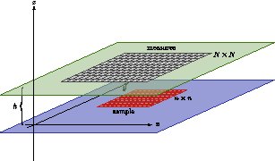
            <caption align="bottom"><strong>Figure
	5. </strong>Schematic view of the experimental setup</caption>
            <tr align="center">
              <td>
                <table>
                  <tr>
                    <td xmlns="" style="height:3px;" align="center">
                      <img xmlns="http://www.w3.org/1999/xhtml" alt="IMG/schema-dispositif.png" src="IMG/schema-dispositif.png"/>
                    </td>
                  </tr>
                </table>
              </td>
            </tr>
          </table>
        </div>
        <p>Figure <a title="Source recovery problems" href="./uid58.html#uid61">5</a>  presents a schematic view of the experimental setup: the sample lie on a horizontal plane at height 0 and its support is included in a rectangle. The vertical component <span class="math"><math xmlns="http://www.w3.org/1998/Math/MathML"><msub><mi>B</mi><mi>z</mi></msub></math></span> of the field produced by the sample is measured on points of a horizontal <span class="math"><math xmlns="http://www.w3.org/1998/Math/MathML"><mrow><mi>N</mi><mo>×</mo><mi>N</mi></mrow></math></span> rectangular grid at height <span class="math"><math xmlns="http://www.w3.org/1998/Math/MathML"><mi>h</mi></math></span>.</p>
        <p>We set up last year a heuristic procedure to recover regularly spaced dipolar magnetizations, <i>i.e.</i> magnetizations composed of dipoles placed at the points of a regular rectangular <span class="math"><math xmlns="http://www.w3.org/1998/Math/MathML"><mrow><mi>n</mi><mo>×</mo><mi>n</mi></mrow></math></span> grid. The latter seems general enough a model class to approximate magnetizations commonly
encountered in samples. However, for reasons of computational complexity,
<span class="math"><math xmlns="http://www.w3.org/1998/Math/MathML"><mi>n</mi></math></span> is significantly smaller than <span class="math"><math xmlns="http://www.w3.org/1998/Math/MathML"><mi>N</mi></math></span> which limits
the power of the model.
Each dipole of the <span class="math"><math xmlns="http://www.w3.org/1998/Math/MathML"><mrow><mi>n</mi><mo>×</mo><mi>n</mi></mrow></math></span> grid is determined by the 3 components of its moment, thus the magnetization can be represented by a real <span class="math"><math xmlns="http://www.w3.org/1998/Math/MathML"><mrow><mn>3</mn><msup><mi>n</mi><mn>2</mn></msup></mrow></math></span>-vector. If we denote by <span class="math"><math xmlns="http://www.w3.org/1998/Math/MathML"><mi>A</mi></math></span> the matrix of the operator that maps such a vector <span class="math"><math xmlns="http://www.w3.org/1998/Math/MathML"><mi>X</mi></math></span> to the vector <span class="math"><math xmlns="http://www.w3.org/1998/Math/MathML"><mi>b</mi></math></span> of measurements (which belongs to <span class="math"><math xmlns="http://www.w3.org/1998/Math/MathML"><msup><mi>ℝ</mi><msup><mi>N</mi><mn>2</mn></msup></msup></math></span>), we want
to find <span class="math"><math xmlns="http://www.w3.org/1998/Math/MathML"><mi>X</mi></math></span> such that <span class="math"><math xmlns="http://www.w3.org/1998/Math/MathML"><mrow><mi>A</mi><mi>X</mi></mrow></math></span> is close to <span class="math"><math xmlns="http://www.w3.org/1998/Math/MathML"><mi>b</mi></math></span>. For computational simplicity,
we use a Euclidean criterion <span class="math"><math xmlns="http://www.w3.org/1998/Math/MathML"><msub><mrow><mo>∥</mo><mi>A</mi><mi>X</mi><mo>-</mo><mi>b</mi><mo>∥</mo></mrow><mn>2</mn></msub></math></span>, which reduces the problem to a singular value decomposition of <span class="math"><math xmlns="http://www.w3.org/1998/Math/MathML"><mi>A</mi></math></span>. The inverse problem being ill-posed,
<span class="math"><math xmlns="http://www.w3.org/1998/Math/MathML"><mi>A</mi></math></span> is poorly conditioned and we must resort to a
regularization technique. The one we developed initially has been
based on iteratively cropping the support of <span class="math"><math xmlns="http://www.w3.org/1998/Math/MathML"><mi>b</mi></math></span>, using a threshold on the intensity of the dipoles at each step, so as to reduce the number of active components in <span class="math"><math xmlns="http://www.w3.org/1998/Math/MathML"><mi>b</mi></math></span>. Preliminary experiments were performed last year on synthetic data and also on a real example (Lonar spherule).</p>
        <p>This year, we performed more systematic experiments on real data (namely Allende chondrules and Hawaian basalt) provided by the SQUID scanning microscope at MIT lab. Cropping the support of <span class="math"><math xmlns="http://www.w3.org/1998/Math/MathML"><mi>b</mi></math></span> using thresholding
has proved efficient to improve ill-conditioning
for samples with localized support embedded in the slab (<i>e.g.</i>, chondrules). On the other hand, when the support of the sample is spread out (<i>e.g.</i>, Hawaian basalt), the reduction of active components of <span class="math"><math xmlns="http://www.w3.org/1998/Math/MathML"><mi>b</mi></math></span>
was insignificant. We used this inversion procedure to
estimate the net moment. The importance of the latter has been emphasized by the geophysicists at MIT for at least two reasons: firstly it yields important geological information on the sample in particular to estimate the magnitude of the ambient magnetic field at the time the rock was formed. Secondly, it may
to some extent be measured independently, using a magnetometer, thereby allowing one to cross-validate the approach. A third, computational reason is that knowledge of the net moment should pave the way to a numerically stable reconstruction of an equivalent unidirectional magnetization. The support of the latter would provide us with valuable information to test for unidirectionality of the true magnetization, which is an important question to physicists.</p>
        <p>When the support can be significantly shrunk while keeping the residue small (<i>i.e.</i>, explaining the data satisfactorily), estimates of the net moment based on the dipolar model obtained by inversion seem to be good. They apparently supersede the measurements by magnetometers as well as by dipole fitting procedures set up at MIT. It is interesting to notice that the magnetization obtained by our inversion procedure, either before or after shrinking the support, often does not resemble the true magnetization, even when it yields correct moment and field. This can be seen on synthetic examples and may be surmised on real data, thereby confirming that recovering the net moment and recovering the magnetization are rather different problems, the latter being
considerably more ill-posed than the former.</p>
        <p>One specific difficulty with chondrule-type examples has been
to account for their thickness: they are indeed small spheres and their
3-D character cannot be completely ignored. In order to use the inversion procedure set up in the plane, we investigated the following question.
Assume that the sample has some thickness, but small enough that the
magnetization at a point <span class="math"><math xmlns="http://www.w3.org/1998/Math/MathML"><mrow><mi>P</mi><mo>=</mo><mo>(</mo><mi>x</mi><mo>,</mo><mi>y</mi><mo>,</mo><mi>z</mi><mo>)</mo></mrow></math></span> inside the sample depends only
on <span class="math"><math xmlns="http://www.w3.org/1998/Math/MathML"><mi>x</mi></math></span> and <span class="math"><math xmlns="http://www.w3.org/1998/Math/MathML"><mi>y</mi></math></span> (possibly weighted by some function that depends only on <span class="math"><math xmlns="http://www.w3.org/1998/Math/MathML"><mi>z</mi></math></span>), <i>i.e.</i> that it is of the form <span class="math"><math xmlns="http://www.w3.org/1998/Math/MathML"><mrow><mi>m</mi><mo>(</mo><mi>x</mi><mo>,</mo><mi>y</mi><mo>)</mo><mi>φ</mi><mo>(</mo><mi>z</mi><mo>)</mo></mrow></math></span>. If we consider a (truly) planar magnetization with the same distribution <span class="math"><math xmlns="http://www.w3.org/1998/Math/MathML"><mrow><mi>m</mi><mo>(</mo><mi>x</mi><mo>,</mo><mi>y</mi><mo>)</mo></mrow></math></span> but on a plane lying
at some nonzero height <span class="math"><math xmlns="http://www.w3.org/1998/Math/MathML"><mi>ε</mi></math></span>, how to choose <span class="math"><math xmlns="http://www.w3.org/1998/Math/MathML"><mi>ε</mi></math></span> so as to produce a field at height <span class="math"><math xmlns="http://www.w3.org/1998/Math/MathML"><mi>h</mi></math></span> which is closest to the field produced by the thick magnetization? This has been the object of the internship of Olga Permiakova who used local expansion of the dipole-to-field map (see her report (<a href="http://www-sop.inria.fr/apics/IMPINGE/Documents/Report_Permiakova_Olga.pdf">http://www-sop.inria.fr/apics/IMPINGE/Documents/Report_Permiakova_Olga.pdf</a> )). An article is being written on this subject.</p>
        <p>The case where the magnetization is flat but spread out on the sample
is more difficult. First of all, the computational effort becomes significant and led us to use the cluster at Inria Sophia Antipolis.
We succeeded in obtaining full inversions for the Hawaian basalt. The residue (approximation error) is moderate but not impressively small,
which indicates that we reach the limit of modeling
magnetizations by a regular grid of dipoles. However the computation of the moment compares favorably with estimates previously obtained by a different technique at MIT lab. Still, using a cluster and two days of evaluation to obtain a coarse estimate of the net moment of a sample is rather inefficient and calls for new investigations.</p>
        <p>We also experimented an alternative regularization procedure, based on <span class="math"><math xmlns="http://www.w3.org/1998/Math/MathML"><msup><mi>L</mi><mn>2</mn></msup></math></span> minimization under <span class="math"><math xmlns="http://www.w3.org/1998/Math/MathML"><msup><mi>L</mi><mn>1</mn></msup></math></span> penalty as solved by the SALSA algorithm. Such methods
are quite popular today for sparse recovery. However,
the computational load, as well as the quality of the results, do not differ significantly from those obtained previously.</p>
        <p>We now develop new methods in order to estimate the net moment of the magnetization, based on improvements of previously used Fourier techniques, and recently we reformulated the problem with the help of Kelvin transforms.
It has been realized that the success of net moment recovery hinges on
the ability to extrapolate the measurements. In particular, we managed to considerably improve previous estimates by means of data extension based on dipolar field asymptotics.</p>
        <p>In the course of inverting the field map, we singled out magnetizations which are numerically (almost) silent from above though not from below. This illustrates how ill-posed (unstable) the problem, as theory predicts that no compactly supported magnetization can be exactly silent from above without being also exactly silent from below. Although such magnetizations seem to have small moment and therefore do not endanger the possibility of recovering the net moment,
their existence is certainly an obstacle to inversion of the field map without extra measurements or hypotheses (<i>e.g.</i>, measuring from below or
assuming unidirectionality).</p>
        <p>In the course of the doctoral work by D. Ponomarev,
the study of the 2D spectral decomposition of the truncated Poisson operator
has been undertaken. It is a simplified version of the relation between the magnetization and the magnetic potential.
We considered several formulations in terms of singular integral equations and matrix Riemann-Hilbert problems, and focused on finding closed form solutions for various approximations of the Poisson operator in terms of
a the ratio between the distance <span class="math"><math xmlns="http://www.w3.org/1998/Math/MathML"><mi>h</mi></math></span> to the measurement plane
and the sample support size.</p>
        <p>Lately, Apics became a partner of the
ANR project MagLune, dealing with Lunar magnetism, a
in collaboration with the Geophysics and Planetology Department of Cerege,
CNRS, Aix-en-Provence, see section <a title="National Initiatives" href="./uid87.html#uid89">
	8.2.2</a> . The research is
just starting, and will focus on computing net moments of lunar rock samples
collected by NASA.</p>
      </div>
      <!--FIN du corps du module-->
      <br/>
      <div class="bottomNavigation">
        <div class="tail_aucentre">
          <a href="./uid56.html" accesskey="P"><img style="align:bottom; border:none" alt="previous" src="../static/img/icons/previous_motif.jpg"/> Previous | </a>
          <a href="./uid0.html" accesskey="U"><img style="align:bottom; border:none" alt="up" src="../static/img/icons/up_motif.jpg"/>  Home</a>
          <a href="./uid63.html" accesskey="N"> | Next <img style="align:bottom; border:none" alt="next" src="../static/img/icons/next_motif.jpg"/></a>
        </div>
        <br/>
      </div>
    </div>
  </body>
</html>