Section: New Results

Compiling Probabilistic Programs Onto Reconfigurable Logic Using Stochastic Arithmetic

Participants : Emmanuel Mazer, Marvin Faix.

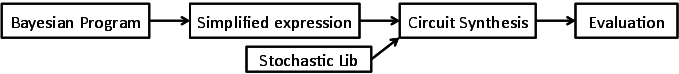
It is of great interest to perform light weight probabilistic inferences for applications such as sensor fusion. Our goal is to design systems to perform these inferences without using a Von Newman machine nor standard floating point arithmetic. By addressing the core of how computations are made, we can explore the tradeoffs between system precision with power consumption and computation time, enabling artificial systems with limited resources, such as mobile and embedded systems, to better operate under uncertainty. Figure 15 illustrates the tool-chain, which starts from the specification of the Bayesian Program in Bayesian programming language , and evaluates it on a reconfigurable device.

This study is part of BAMBI (Bottom-up Approaches to Machines dedicated to Bayesian Inference, www.bambi-fet.eu ) : a European collaborative research project relying on the theory of Bayesian inference to understand the natural cognition and aiming at designing bio-inspired computing devices.

A Bayesian machine has probability distributions as inputs and returns a probability distribution as output. It is defined by a joint probability distribution on a set of discrete and finite variables: $P(M\wedge D\wedge L)$. Where $M,D$ and $L$ are themselves conjunctions of variables, for example $D=D_1\wedge ...\wedge D_k$. We define the soft evidences on the variables $D_k$ as the probability distribution $\tilde{P}\left(D_k\right)$. These soft evidences will be the inputs of the Bayesian machine.

So, given the soft evidences $\tilde{P}\left(D_k\right)$ and the joint distribution $P(M\wedge D\wedge L)$, the machine will fulfil the specification if it computes:

with

$Z=\sum _M(\sum _{D_1}\tilde{P}\left(D_1\right)...\sum _{D_k}\tilde{P}\left(D_k\right)\sum _{L}P(M\wedge D\wedge L)$

In other words the machine computes a soft inference based on the joint distribution $P(M\wedge D\wedge L)$ .

A modified version of the probabilistic language ProBT is used to specify the machine: the joint distribution, the output and the inputs are specified with this language (A free version of ProBT is available at http://www.probayes.com/fr/Bayesian-Programming-Book/ and the version with soft evidence will be placed on www.bambi-fet.eu before the NIPS conference ). The next program is an example of a simple specification using the Python bindings of ProBT.

#import the ProBT bindings

from pypl import *

#define the variables

dim3 = plIntegerType(0,2)

D1 = plSymbol(D1,dim3)

D2 = plSymbol(D2,dim3)

M= plSymbol(M,dim3)

#define the distribution on M

PM= plProbTable(M,[0.8,0.1,0.1])

#define a conditional distribution on D1

PD1_k_M = plDistributionTable(D1,M)

PD1_k_M.push(plProbTable(D1,[0.5,0.2,0.3]),0)

PD1_k_M.push(plProbTable(D1,[0.5,0.3,0.2]),1)

PD1_k_M.push(plProbTable(D1,[0.4,0.3,0.3]),2)

#define a conditional distribution on D2

PD2_k_M = plDistributionTable(D2,M)

PD2_k_M.push(plProbTable(D2,[0.2,0.6,0.2]),0)

PD2_k_M.push(plProbTable(D2,[0.6,0.3,0.1]),1)

PD2_k_M.push(plProbTable(D2,[0.3,0.6,0.1]),2)

#define the joint distribution

model=plJointDistribution(PM*PD1_k_M*PD2_k_M)

#define the soft evidence variables

model.set_soft_evidence_variables(D1^D2)

#define the output

question=model.ask(M)

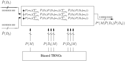
Figure 16 presents the high-level representation of the architecture for the Bayesian Machine. It comprises the main stochastic machine along with the True Random Generators (TRNG), responsible for the generation of the stochastic bit streams for the constants considered in the problem.

The proposed tool-chain is working and accepts any ProBT program with discrete variables as entry. The tool-chain generates a VHDL file which is the description of the stochastic circuit and can be implemented on a FPGA. A Cyclone IV FPGA, from Altera has been targeted as supporting device. A machine has been synthesised to demonstrate the applicability and scalability of the proposed tool-chain. ProBT is also used to compute the exact result using standard arithmetic. This allows to evaluate the results given by FPGA with the synthesised VHDL program.

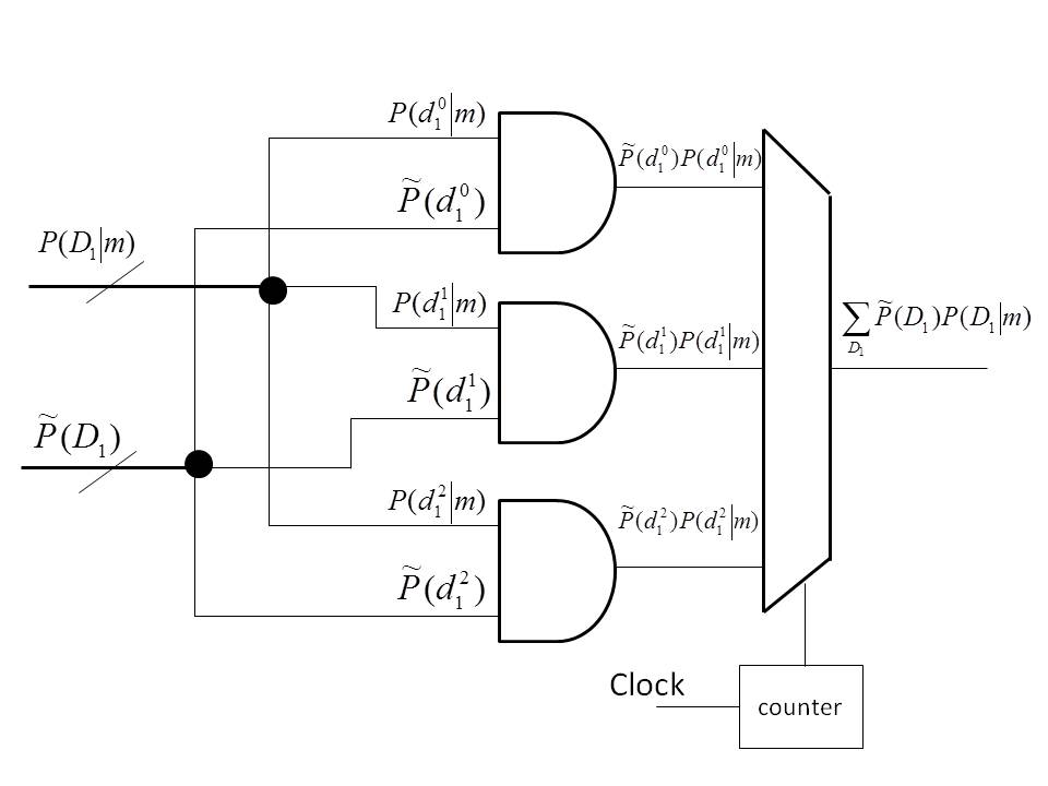
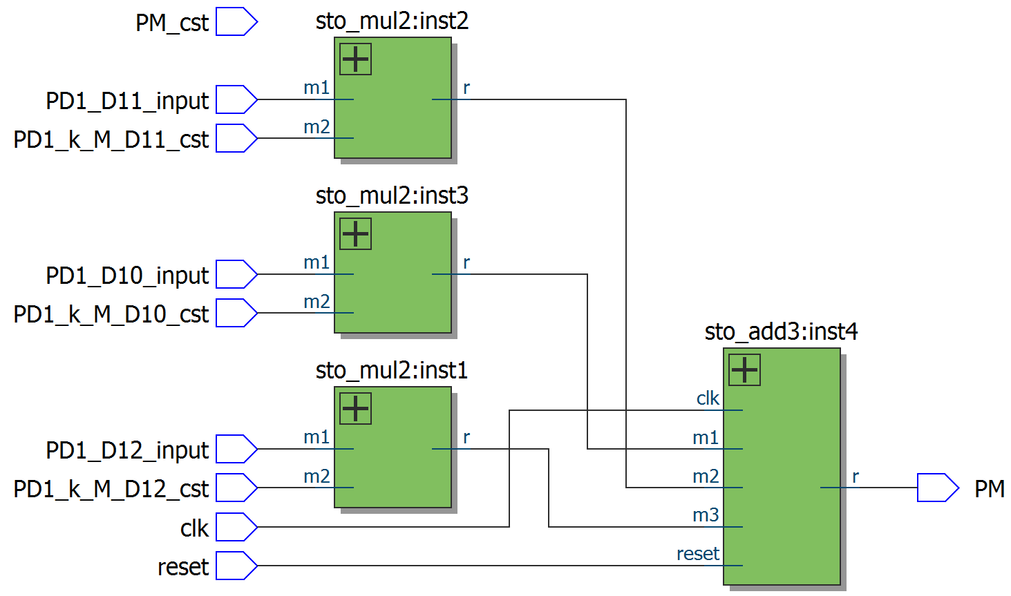
Figure 17 (right) shows the RTL generated by the synthesis tool, where it is possible to identify the connections between the components, corresponding to the circuit in Figure 17 (left). This circuit was implemented using 6 Logic Elements. The circuit was tested with bit streams integrated over $2^{31}$ to do the conversion from stochastic to binary.

The proposed tool-chain is working and accepts any ProBT program with discrete variables as entry. The tool-chain generates a VHDL file which is the description of the stochastic circuit and can be implemented on a FPGA. A Cyclone IV FPGA, from Altera has been targeted as supporting device. A machine has been synthesised to demonstrate the applicability and scalability of the proposed tool-chain.

ProBT is also used to compute the exact result using standard arithmetic. This allows to evaluate the results given by FPGA with the synthesised VHDL program.

Figure 17 (right) shows the RTL generated by the synthesis tool, where it is possible to identify the connections between the components, corresponding to the circuit in Figure 17 (left). This circuit was implemented using 6 Logic Elements. The circuit was tested with bit streams integrated over $2^{31}$ to do the conversion from stochastic to binary.

We are now focusing on solving the time dilution problem by introducing memory in the architecture. Then we will make an attempt to build a filter with similar ideas by re-fitting the output into the initial joint distribution.