Section: New Software and Platforms

New Softwares

Hope : High Order Program for Energy

This software is focused on the numerical simulation of 2D transport equation using fully deterministic methods (high order finite difference solvers, semi-Lagrangian methods).

Numerical simulation of guiding center model [9]

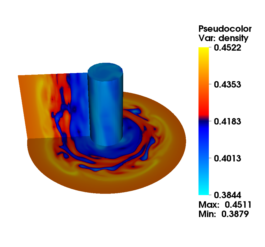
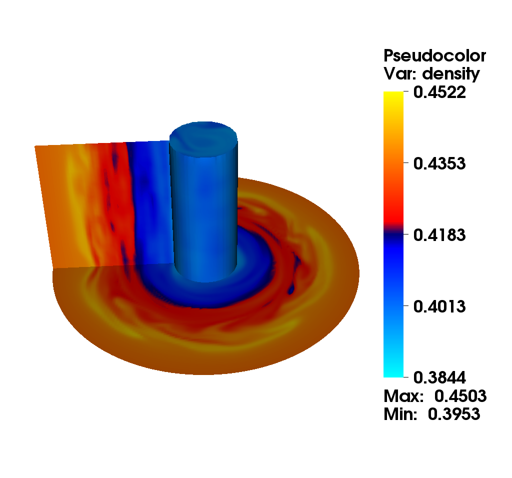
We consider the diocotron instability for an annular electron layer. This plasma instability is created by two sheets of charge slipping past each other and is the analog of the Kelvin-Helmholtz instability in fluid mechanics. We propose a comparison of two different numerical methods : the mixed method (top): this method uses alternatively a semi-Lagrangian and finite difference method with fifth order Hermite WENO reconstruction. The choice is made automatically according to a good preservation of mass (the finite difference method is conservative). the semi-Lagrangian (bottom): this method is based on a cubic spline interpolation for the reconstruction of the distribution function.

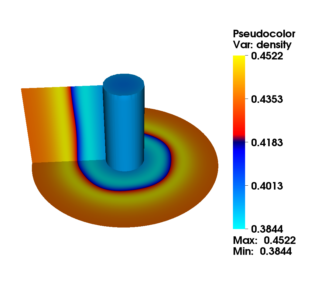
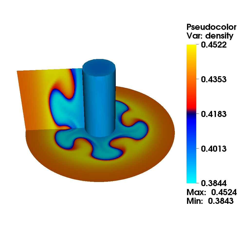
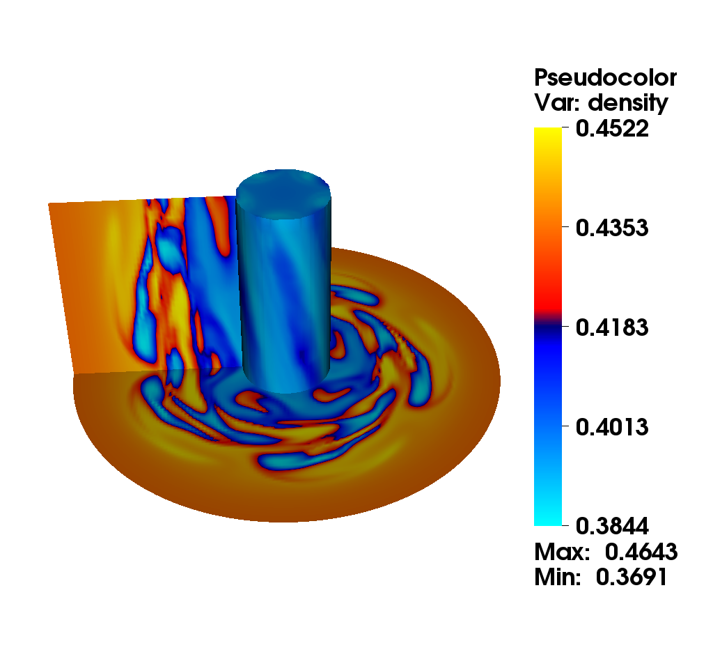
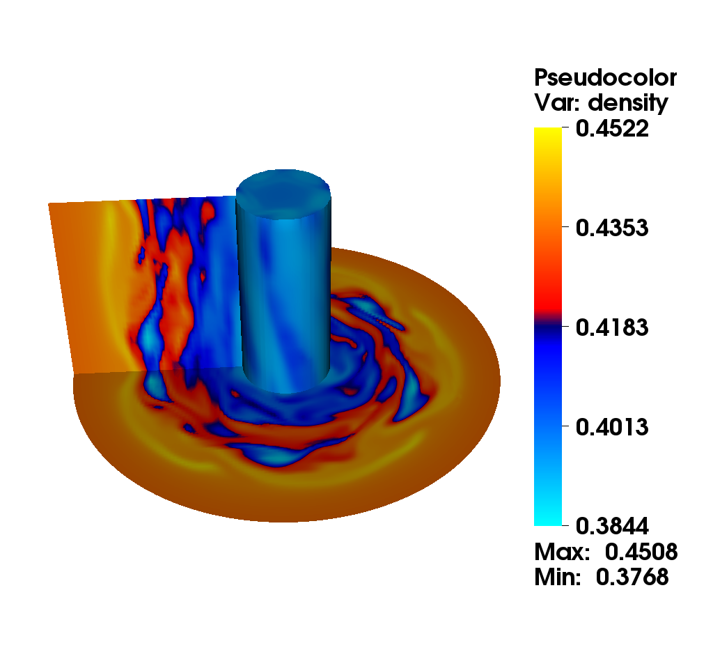
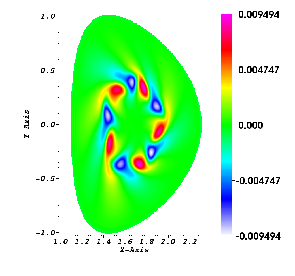
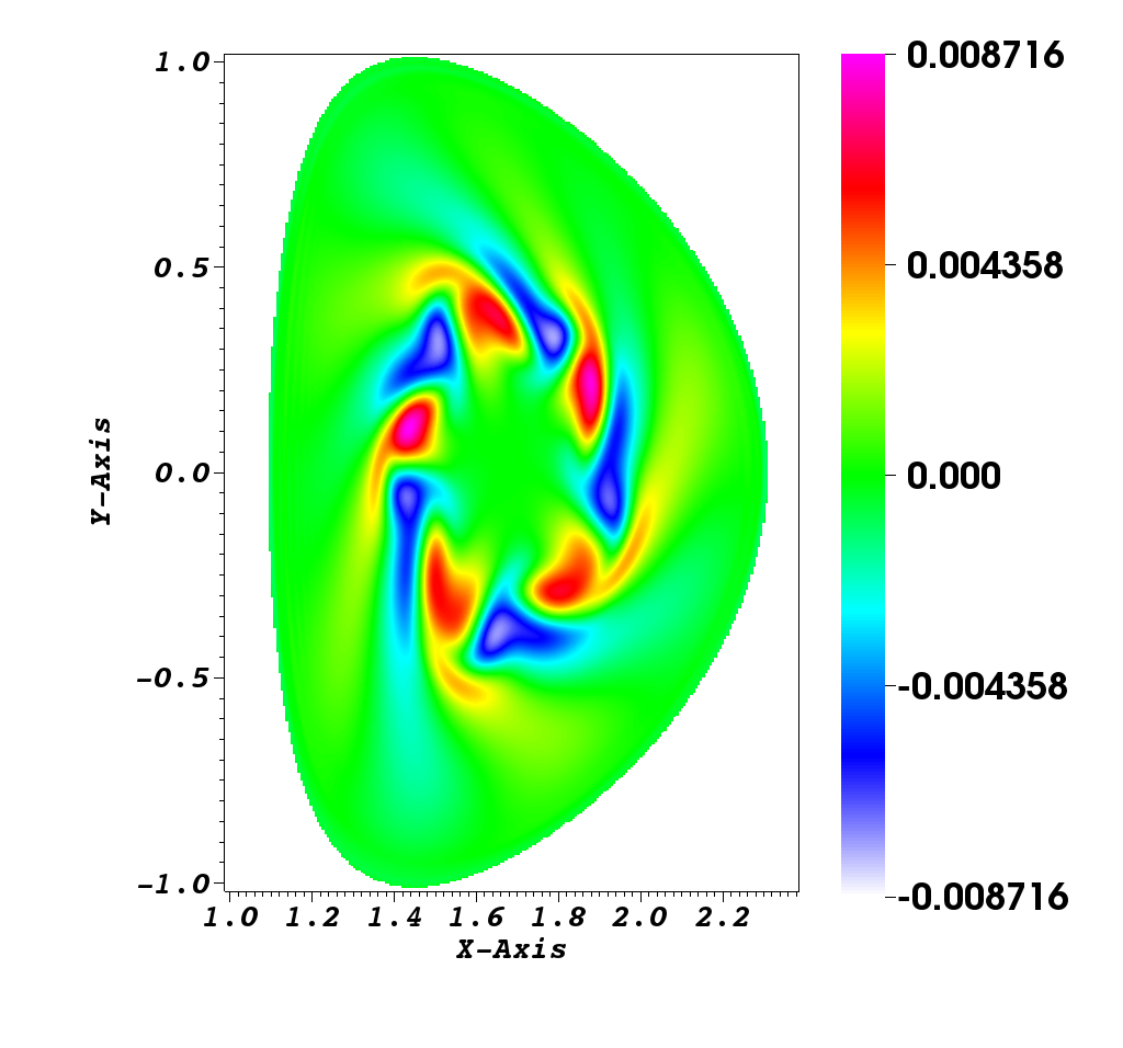
Numerical simulation in a D shape [9]

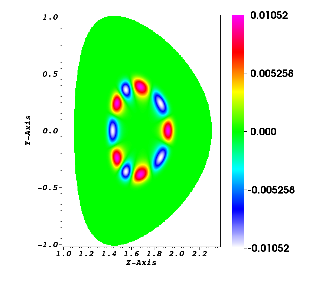
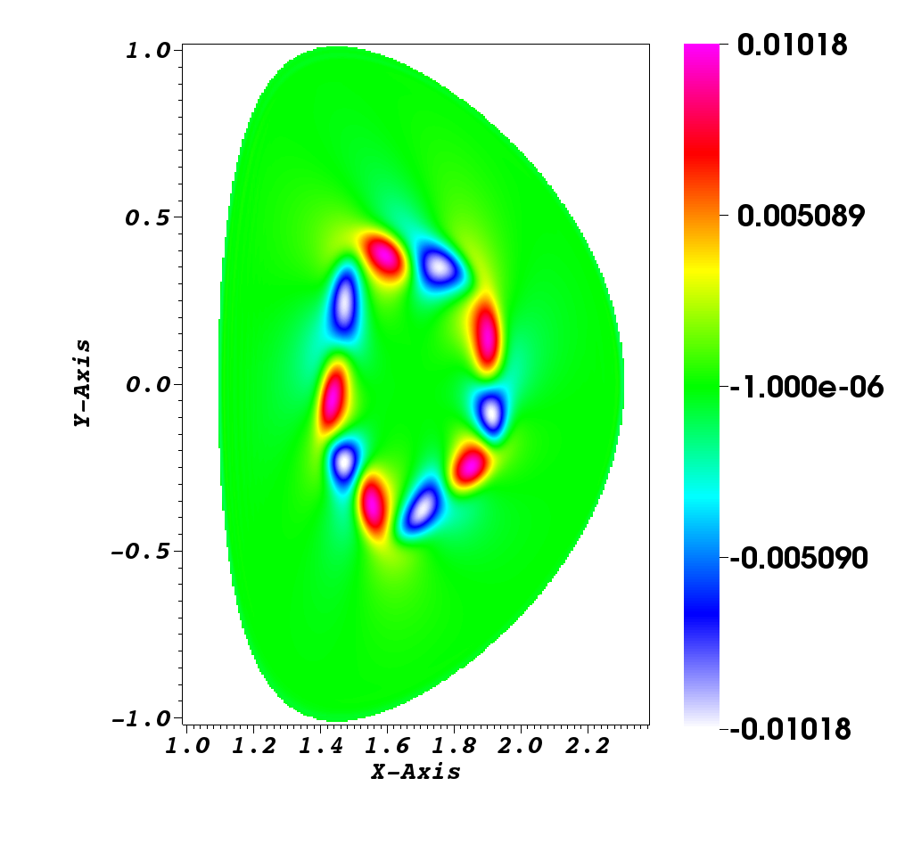
This simulation illustrates an instability development of the solution to the guiding-center model in a D-shaped domain. We present the difference between the perturbed density and the steady state density. An instability develops and generates small filaments. It correspond to the motion of the density in the transverse plane of the tokamak.

Figure 2 illustrates the evolution of density governed by the guiding-center model. We present the difference between the perturbed density and the steady state density, i.e. $\delta \rho \left(t\right)=\overline{\rho }\left(t\right)-{\overline{\rho }}_0$. We observe that the difference of density $\delta \rho$ revolves, and small filaments appear at time $t=200$. Until the time $t=300$, we can clearly identify the filaments.

Towards 4D numerical simulations

The discretization of the Drift-Kinetic model can be developed very similarly as the one for the guiding-center model. Here, we present some principle discretization steps.

The Vlasov equation of system can be split into three equations :

$\left\{\begin{array}{c}{\displaystyle \frac{\partial f}{\partial t}+𝐔·{\nabla }_{{𝐱}_{\perp }}f=0,}\hfill \\ {\displaystyle \frac{\partial f}{\partial t}+v_{\parallel }{\partial }_{z}f=0,}\hfill \\ {\displaystyle \frac{\partial f}{\partial t}+E_{\parallel }{\partial }_{v_{\parallel }}f=0.}\hfill \end{array}\right.$

This test represents a snapshot of the charge density when an instability occurs (ion turbulence simulation). This simulation has been realized by different methods but in cylindrical coordinates, here we perform numerical simulation in Cartesian coordinates on a uniform grid. The discretization of the Drift-Kinetic model can be developed very similarly as the one for the guiding-center model.