Section: Research Program

Stochastic models

The second axis in the theoretical developments of the Regularity team aims at defining and studying stochastic processes for which various aspects of the local regularity may be prescribed.

Multifractional Brownian motion

One of the simplest stochastic process for which some kind of control over the Hölder exponents is possible is probably fractional Brownian motion (fBm). This process was defined by Kolmogorov and further studied by Mandelbrot and Van Ness, followed by many authors. The so-called “moving average” definition of fBm reads as follows:

where $𝕎$ denotes the real white noise. The parameter $H$ ranges in $(0,1)$, and it governs the pointwise regularity: indeed, almost surely, at each point, both the local and pointwise Hölder exponents are equal to $H$.

Although varying $H$ yields processes with different regularity, the fact that the exponents are constant along any single path is often a major drawback for the modeling of real world phenomena. For instance, fBm has often been used for the synthesis natural terrains. This is not satisfactory since it yields images lacking crucial features of real mountains, where some parts are smoother than others, due, for instance, to erosion.

It is possible to generalize fBm to obtain a Gaussian process for which the pointwise Hölder exponent may be tuned at each point: the multifractional Brownian motion (mBm) is such an extension, obtained by substituting the constant parameter $H\in (0,1)$ with a regularity function $H:{ℝ}_{+}\to (0,1)$.

mBm was introduced independently by two groups of authors: on the one hand, Peltier and Levy-Vehel [29] defined the mBm $\{X_t;t\in {ℝ}_{+}\}$ from the moving average definition of the fractional Brownian motion, and set:

On the other hand, Benassi, Jaffard and Roux [45] defined the mBm from the harmonizable representation of the fBm, i.e.:

where $\widehat{𝕎}$ denotes the complex white noise.

The Hölder exponents of the mBm are prescribed almost surely: the pointwise Hölder exponent is ${\alpha }_X\left(t\right)=H\left(t\right)\wedge {\alpha }_H\left(t\right)$ a.s., and the local Hölder exponent is ${\tilde{\alpha }}_X\left(t\right)=H\left(t\right)\wedge {\tilde{\alpha }}_H\left(t\right)$ a.s. Consequently, the regularity of the sample paths of the mBm are determined by the function $H$ or by its regularity. The multifractional Brownian motion is our prime example of a stochastic process with prescribed local regularity.

The fact that the local regularity of mBm may be tuned via a functional parameter has made it a useful model in various areas such as finance, biomedicine, geophysics, image analysis, .... A large number of studies have been devoted worldwide to its mathematical properties, including in particular its local time. In addition, there is now a rather strong body of work dealing the estimation of its functional parameter, i.e. its local regularity. See http://regularity.saclay.inria.fr/theory/stochasticmodels/bibliombm for a partial list of works, applied or theoretical, that deal with mBm.

Self-regulating processes

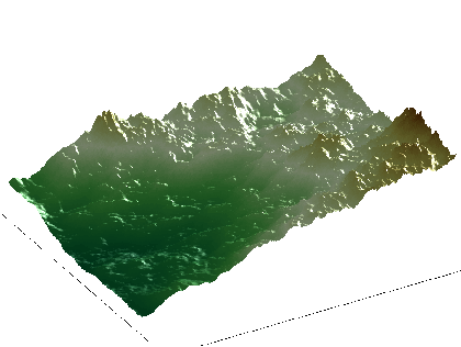
We have recently introduced another class of stochastic models, inspired by mBm, but where the local regularity, instead of being tuned “exogenously”, is a function of the amplitude. In other words, at each point $t$, the Hölder exponent of the process $X$ verifies almost surely ${\alpha }_X\left(t\right)=g\left(X\left(t\right)\right)$, where $g$ is a fixed deterministic function verifying certain conditions. A process satisfying such an equation is generically termed a self-regulating process (SRP). The particular process obtained by adapting adequately mBm is called the self-regulating multifractional process [3] . Another instance is given by modifying the Lévy construction of Brownian motion [4] . The motivation for introducing self-regulating processes is based on the following general fact: in nature, the local regularity of a phenomenon is often related to its amplitude. An intuitive example is provided by natural terrains: in young mountains, regions at higher altitudes are typically more irregular than regions at lower altitudes. We have verified this fact experimentally on several digital elevation models [8] . Other natural phenomena displaying a relation between amplitude and exponent include temperatures records and RR intervals extracted from ECG [9] .

To build the SRMP, one starts from a field of fractional Brownian motions $B(t,H)$, where $(t,H)$ span $[0,1]\times [a,b]$ and $0<a<b<1$. For each fixed $H$, $B(t,H)$ is a fractional Brownian motion with exponent $H$. Denote:

the affine rescaling between ${\alpha }^{\text{'}}$ and ${\beta }^{\text{'}}$ of an arbitrary continuous random field over a compact set $K$. One considers the following (stochastic) operator, defined almost surely:

where $\alpha \le {\alpha }^{\text{'}}<{\beta }^{\text{'}}\le \beta$, $\alpha$ and $\beta$ are two real numbers, and ${\alpha }^{\text{'}},{\beta }^{\text{'}}$ are random variables adequately chosen. One may show that this operator is contractive with respect to the sup-norm. Its unique fixed point is the SRMP. Additional arguments allow to prove that, indeed, the Hölder exponent at each point is almost surely $g\left(t\right)$.

An example of a two dimensional SRMP with function $g\left(x\right)=1-x^2$ is displayed on figure 1 .

We believe that SRP open a whole new and very promising area of research.

Multistable processes

Non-continuous phenomena are commonly encountered in real-world applications, e.g. financial records or EEG traces. For such processes, the information brought by the Hölder exponent must be supplemented by some measure of the density and size of jumps. Stochastic processes with jumps, and in particular Lévy processes, are currently an active area of research.

The simplest class of non-continuous Lévy processes is maybe the one of stable processes [56] . These are mainly characterized by a parameter $\alpha \in (0,2]$, the stability index ($\alpha =2$ corresponds to the Gaussian case, that we do not consider here). This index measures in some precise sense the intensity of jumps. Paths of stable processes with $\alpha$ close to 2 tend to display “small jumps”, while, when $\alpha$ is near 0, their aspect is governed by large ones.

In line with our quest for the characterization and modeling of various notions of local regularity, we have defined multistable processes. These are processes which are “locally” stable, but where the stability index $\alpha$ is now a function of time. This allows to model phenomena which, at times, are “almost continuous”, and at others display large discontinuities. Such a behaviour is for instance obvious on almost any sufficiently long financial record.

More formally, a multistable process is a process which is, at each time $u$, tangent to a stable process [49] . Recall that a process $Y$ is said to be tangent at $u$ to the process $Y_u^{\text{'}}$ if:

where the limit is understood either in finite dimensional distributions or in the stronger sense of distributions. Note $Y_u^{\text{'}}$ may and in general will vary with $u$.

One approach to defining multistable processes is similar to the one developed for constructing mBm [29] : we consider fields of stochastic processes $X(t,u)$, where $t$ is time and $u$ is an independent parameter that controls the variation of $\alpha$. We then consider a “diagonal” process $Y\left(t\right)=X(t,t)$, which will be, under certain conditions, “tangent” at each point $t$ to a process $t\mapsto X(t,u)$.

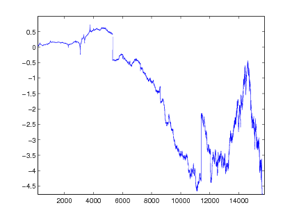
A particular class of multistable processes, termed “linear multistable multifractional motions” (lmmm) takes the following form [11] , [10] . Let $(E,ℰ,m)$ be a $\sigma$-finite measure space, and $\Pi$ be a Poisson process on $E\times ℝ$ with mean measure $m\times ℒ$ ($ℒ$ denotes the Lebesgue measure). An lmmm is defined as:

where $x^{<y>}:=\text{sign}\left(x\right){\left|x\right|}^y$, $a:ℝ\to {ℝ}^{+}$ is a $C^1$ function and $\alpha :ℝ\to (0,2)$ and $h:ℝ\to (0,1)$ are $C^2$ functions.

In fact, lmmm are somewhat more general than said above: indeed, the couple $(h,\alpha )$ allows to prescribe at each point, under certain conditions, both the pointwise Hölder exponent and the local intensity of jumps. In this sense, they generalize both the mBm and the linear multifractional stable motion [57] . From a broader perspective, such multistable multifractional processes are expected to provide relevant models for TCP traces, financial logs, EEG and other phenomena displaying time-varying regularity both in terms of Hölder exponents and discontinuity structure.

Figure 2 displays a graph of an lmmm with linearly increasing $\alpha$ and linearly decreasing $H$. One sees that the path has large jumps at the beginning, and almost no jumps at the end. Conversely, it is smooth (between jumps) at the beginning, but becomes jaggier and jaggier as time evolves.