|
|

|

|
| e-Pub |
Section: Research Program
Inverse problems in Neuroimaging
Many problems in neuroimaging can be framed as forward and inverse problems. For instance, brain population imaging is concerned with the inverse problem that consists in predicting individual information (behavior, phenotype) from neuroimaging data, while the corresponding forward problem boils down to explaining neuroimaging data with the behavioral variables. Solving these problems entails the definition of two terms: a loss that quantifies the goodness of fit of the solution (does the model explain the data well enough ?), and a regularization scheme that represents a prior on the expected solution of the problem. These priors can be used to enforce some properties on the solutions, such as sparsity, smoothness or being piece-wise constant.
Let us detail the model used in typical inverse problem: Let be a neuroimaging dataset as an matrix, where and are the number of subjects under study, and the image size respectively, a set of values that represent characteristics of interest in the observed population, written as matrix, where is the number of characteristics that are tested, and an array of shape that represents a set of pattern-specific maps. In the first place, we may consider the columns of independently, yielding problems to be solved in parallel:
where the vector contains is the row of . As the problem is clearly ill-posed, it is naturally handled in a regularized regression framework:
where is an adequate penalization used to regularize the solution:
with (this formulation particularly highlights the fact that convex regularizers are norms or quasi-norms). In general, only one or two of these constraints is considered (hence is enforced with a non-zero coefficient):
-
When only (LASSO), and to some extent, when only (elastic net), the optimal solution is (possibly very) sparse, but may not exhibit a proper image structure; it does not fit well with the intuitive concept of a brain map.
-
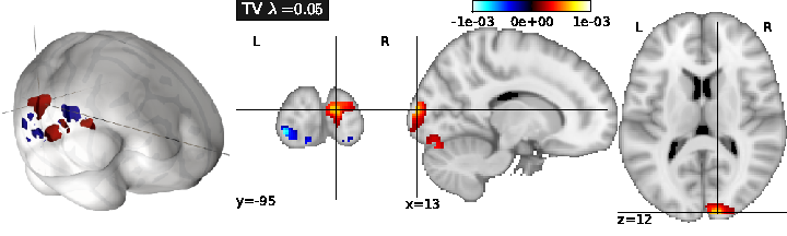
Total Variation regularization (see Fig. 1) is obtained for ( only), and typically yields a piece-wise constant solution. It can be associated with Lasso to enforce both sparsity and sparse variations.
-
Smooth lasso is obtained with ( and only), and yields smooth, compactly supported spatial basis functions.
Note that, while the qualitative aspect of the solutions are very different, the predictive power of these models is often very close.
|
The performance of the predictive model can simply be evaluated as the amount of variance in fitted by the model, for each . This can be computed through cross-validation, by learning on some part of the dataset, and then estimating using the remainder of the dataset.
This framework is easily extended by considering
-
Grouped penalization, where the penalization explicitly includes a prior clustering of the features, i.e. voxel-related signals, into given groups. This amounts to enforcing structured priors on the problem solution.
-
Combined penalizations, i.e. a mixture of simple and group-wise penalizations, that allow some variability to fit the data in different populations of subjects, while keeping some common constraints.
-
Logistic and hinge regression, where a non-linearity is applied to the linear model so that it yields a probability of classification in a binary classification problem.
-
Robustness to between-subject variability to avoid the learned model overly reflecting a few outlying particular observations of the training set. Note that noise and deviating assumptions can be present in both and
-
Multi-task learning: if several target variables are thought to be related, it might be useful to constrain the estimated parameter vector to have a shared support across all these variables.
For instance, when one of the variables is not well fitted by the model, the estimation of other variables may provide constraints on the support of and thus, improve the prediction of .