Section: New Results

Inverse problems for Poisson-Laplace equations

Participants : Laurent Baratchart, Sylvain Chevillard, Juliette Leblond, Jean-Paul Marmorat, Konstantinos Mavreas.

Inverse magnetization issues from planar data

This work has been carried out in the framework of the Inria Associate Team Impinge , comprising Cauê Borlina, Eduardo Andrade Lima and Benjamin Weiss from the Earth Sciences department at MIT (Boston, USA) and Douglas Hardin, Edward Saff and Cristobal Villalobos from the Mathematics department at Vanderbilt University (Nashville, USA).

The overall goal of Impinge was to determine magnetic properties of rock samples (e.g. meteorites or stalactites), from weak field measurements close to the sample that can nowadays be obtained using SQUIDs (superconducting quantum interference devices). Depending on the geometry of the rock sample, the magnetization distribution can either be considered to lie in a plane or in a parallelepiped of thickness $r$. Some of our results apply to both frameworks (the former appears as a limiting case when $r$ goes to 0), while others concern the 2-D case and have no 3-D counterpart as yet.

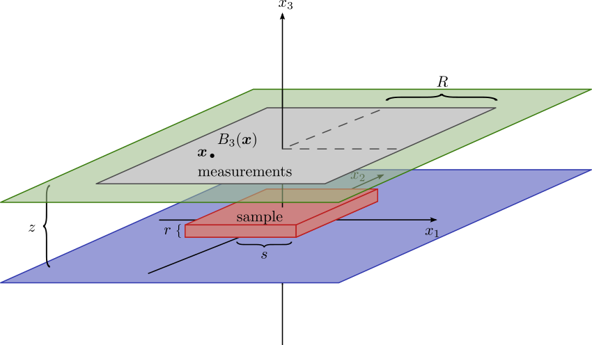
Figure 3 presents a schematic view of the experimental setup: the sample lies on a horizontal plane at height 0 and its support is included in a parallelepiped. The vertical component $B_3$ of the field produced by the sample is measured in points of a horizontal square at height $z$.

We pursued our research efforts towards designing algorithms for net moment recovery. The net moment is the integral of the magnetization over its support, and it is a valuable piece of information to physicists which has the advantage of being determined solely by the field: whereas two different magnetizations can generate the same field, the net moment depends only on the field and not on which magnetization produced it. Hence the goal may be described as to build a numerical magnetometer, capable of analyzing data close to the sample. This is in contrast to classical magnetometers which regard the latter as a single dipole, an approximation which is only valid away from the sample and is not suitable to handle weak fields which get quickly blurred by ambient magnetic sources if one measures the field at a distance from the sample.

The first approach consists in using the fact that the integral of $B_3$ against polynomials of order less or equal to 1 on some domains symmetric with respect to the origin provides an estimate of the net moment, asymptotically when $R$ grows large [20], [72]. This year, on the one hand, we conducted with our colleagues at MIT a campaign of fairly systematic tests (with various sensitivity parameters for the sensor, step size between measurement points, overall size of the measurement rectangle, etc.) to observe how our method behaves on true data. The results are overall very good when the signal-to-noise ratio is not poor; however, this revealed a few situations where the observed asymptotics does not fit the theoretical one, and we have currently no clue of the reason of this phenomenon (is it a manipulation error on some of the samples of our campaign? a bug in our implementation? a noise on the data with a surprisingly large effect on the asymptotic? the fact that the asymptotic regime was not yet reached?) Understanding this phenomenon is still an on-going work. On the other hand, we spotted in the literature approaches that are somehow similar to ours: they compute the same integral, but on the whole plane, and try to account for the finiteness of the measurement rectangle by more or less heuristic methods. As the finiteness of the rectangle is built-in in our approach (we exploit the fact the nature of the asymptotic behavior with respect to $R$ is analytically known), we have good hope that our method should compare favorably against its competitors, but we did not conduct systematic tests yet.

The second approach attempts to generalize the previous expansions in the case when $R$ is moderately large (but only in the thin slab framework, modeling the sample as a rectangle). For this purpose, we setup a bounded extremal problem (BEP, see Section 3.3.1) and submitted an article last year on the subject. It has been accepted for publication this year, see [12].

A third approach developed during the previous years was to design an alternate procedure to compute a good linear estimator, dwelling on expansions on a family of piecewise affine functions, with a restricted number of pieces. A key point here is that it is possible to derive explicit formulas for the adjoint operator $B_3^{*}$ (in appropriate $L^2$ spaces) to the operator $B_3$ mapping a magnetization to the vertical component of the field, when applied to polynomials. We derived this year explicit recurrence formulas that allow one to efficiently compute $B_3^{*}$ of a polynomial of any degree in linear time with respect to the number of monomials. We currently only have draft notes of this research.

Concerning full inversion of thin samples, after preliminary experiments on regularization with $L^1$ constraints (a heavy trend in linear inverse problems today to favor sparse solutions), we started studying magnetizations modeled by signed measures. A loop decomposition of silent sources was obtained, which sharpens in 2-D setting the structure theorem of [76]. Moreover, a characterization of equivalent sources having minimal total variation has been obtained when the support of the magnetization is very scattered (namely: purely 1-unrectifiable, which holds in particular for dipolar models) and also for certain magnetizations of physical interest like unidirectional ones. Thus, it seems that constraining the total variation to regularize the recovery process is appropriate in some important cases. The theoretical analysis has shown that the optimum is then always sparse, in that it has Hausdorff dimension at most 1. This stems from the real analyticity of the operators relating the magnetization to the field, which prevents them from assuming constant level on large sets. Moreover, we proved that the argument of the minimum of the regularized criterion $\parallel f-B_3{\mu \parallel }_2^2+\lambda {\parallel \mu \parallel }_{TV}$ is unique; here, $\mu$ is the measure representing the magnetization with respect to which the criterion gets optimized, $f$ is the data and $\lambda >0$ a regularization parameter, while ${\parallel \mu \parallel }_{TV}$ is the total variation of $\mu$. An implementation is currently being set up with promising results, discretization beforehand on a fixed grid. Yet, a deeper understanding on how to adjust the parameters of the method is required. This topic is studied in collaboration with D. Hardin and C. Villalobos from Vanderbilt University. [21].

Besides, we considered a simplified 2-D setup for magnetizations and magnetic potentials (of which the magnetic field is the gradient). When both the sample and the measurement set are parallel intervals, some best approximation issues related to inverse recovery and relevant BEP problems in Hardy classes of holomorphic functions (see Section 3.3.1). Note that, in the present case, the criterion no longer acts on the boundary of the holomorphy domain (namely, the upper half-plane), but on a strict subset thereof, while the constraint acts on the support of the approximating function. Both involve functions in the Hilbert Hardy space of the upper half-plane. This is the subject of ongoing work with E. Pozzi (Department of Mathematics and Statistics, St Louis Univ., St Louis, Missouri, USA).

For magnetizations supported in a volume $\Omega$ with boundary $\partial \Omega$, there is a greater variety of silent sources, since they have much more space to live in. Now, to each magnetization $m$ supported in $\Omega$ there is a unique magnetization supported on $\partial \Omega$ (the balayage of $m$) and producing the same field outside $\Omega$. Thus, describing silent sources supported on $\partial \Omega$ is a way to factor out some of the complexity of the situation. When $m$ is located in the plane, the Hardy-Hodge decomposition introduced in [35] (see Section 3.3.1) was used there to characterize all silent magnetizations from above (resp. below) as being those having no harmonic gradient from below (resp. above) in their decomposition. When $m$ is supported on a closed compact surface, a similar decomposition exists for ${ℝ}^3$-valued vector fields on $\partial \Omega$, (see Section 6.4), that allows us to characterize all magnetizations on $\partial \Omega$ which are silent from outside as being those whose harmonic components satisfy a certain spectral relation for the double layer potential on $\partial \Omega$. The significance and the algorithmic implications of that equation are under study.

Other types of inverse magnetization problems can be tackled using such techniques, in particular global Geomagnetic issues which arise in spherical geometry. In collaboration with C. Gerhards from the Technische Universität Bergakademie Freiberg (Germany), we developed a method to separate the crustal component of the Earth's magnetic field from its core component, if an estimate of the field is known on a subregion of the globe [33]. This assumption is not unrealistic: parts of Australia and of northern Europe are considered as fairly well understood from the magnetostatic view point. We are currently working to test the algorithm against real data, in collaboration with Geophysicists.

Inverse magnetization issues from sparse cylindrical data

The team Factas is a partner of the ANR project MagLune on Lunar magnetism, headed by the Geophysics and Planetology Department of Cerege, CNRS, Aix-en-Provence (see Section 8.2.1). Recent studies let geoscientists think that the Moon used to have a magnetic dynamo for a while. However, the exact process that triggered and fed this dynamo is still not understood, much less why it stopped. The overall goal of the project is to devise models to explain how this dynamo phenomenon was possible on the Moon.

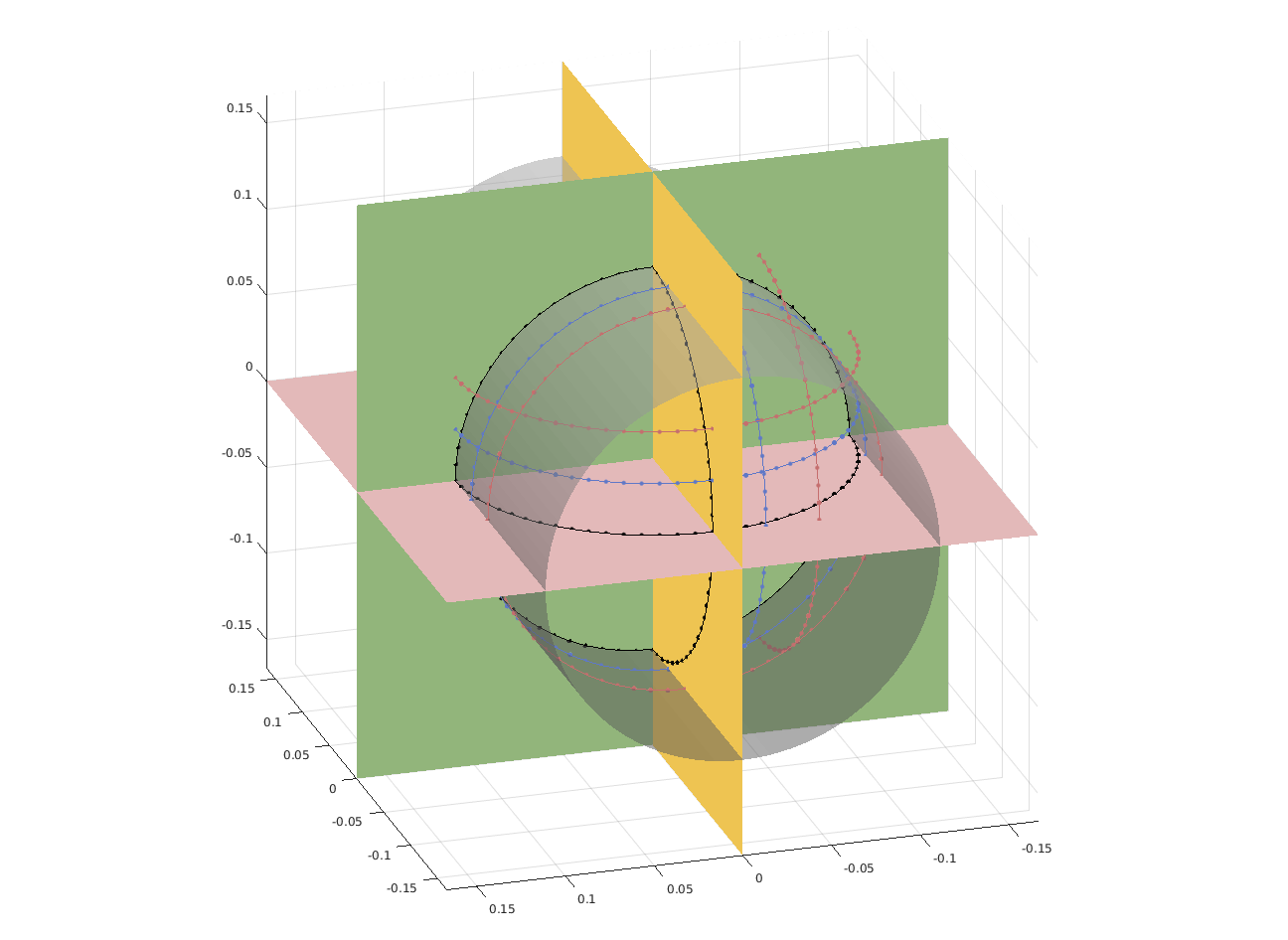
The geophysicists from Cerege went a couple of times to NASA to perform measurements on a few hundreds of samples brought back from the Moon by Apollo missions. The samples are kept inside bags with a protective atmosphere, and geophysicists are not allowed to open the bags, nor to take out samples from NASA facilities. Moreover, the process must be carried out efficiently as a fee is due to NASA by the time when handling these moon samples. Therefore, measurements were performed with some specific magnetometer designed by our colleagues from Cerege. This device measures the components of the magnetic field produced by the sample, at some discrete set of points located on circles belonging to three cylinders (see Figure 4). The objective of Factas is to enhance the numerical efficiency of post-processing data obtained with this magnetometer.

Under the hypothesis that the field can be well explained by a single magnetic pointwise dipole, and using ideas similar to those underlying the FindSources3D tool (see Sections 3.4.2 and 6.1.3), we try to recover the position and the moment of the dipole using the available measurements. This is still on-going work which constitutes the main topic of the PhD thesis of K. Mavreas.

In a given cylinder, using the associated cylindrical system of coordinates, recovering the position of the dipole boils down to determine its height $z$, its radial distance $\rho$ and its azimuth $\phi$. We use a rational approximation technique which, for the circle of measurements at height $h$, gives us an estimate of the complex number $u_h=\frac{1+{\rho }^2+{(h-z)}^2}{\rho }{e}^{i\phi }$, from which $\phi$ is directly obtained. Besides, from the relation $\rho |u_h|=1+{\rho }^2+{(h-z)}^2$, we see that the point $(\rho ,z)$ lies on a circle $C_h$. Therefore, with measurements at three different heights $h_i$ ($i=1,2,3$), we can in principle recover $(\rho ,z)$ as the intersection of the three circles $C_{h_1}$, $C_{h_2}$ and $C_{h_3}$.

In practice, due to the many sources of imprecision (the first of all being that the field is not truly generated by a single dipole), the circles do not all truly intersect. This year, we studied three different strategies to estimate the pseudo-intersection point of the circles. In the plane, for a point $P$ and a circle $C$ of center $O$ and radius $R$, we define $d(P,C)=|\parallel PO\parallel -R|$ where $\parallel ·\parallel$ denotes the Euclidean distance, and $h(P,C)={\parallel PO\parallel }^2-R^2$ and we formulate the problem of finding a pseudo-intersection point between $C_{h_1}$, $C_{h_2}$ and $C_{h_3}$ as either:

1. finding a point $P$ that minimizes $d(P,C_{h_1})+d(P,C_{h_2})+d(P,C_{h_3})$;

2. finding a point $P$ for which $h(P,C_{h_1})=h(P,C_{h_2})=h(P,C_{h_3})$;

3. finding a point $P$ that minimizes $h{(P,C_{h_1})}^2+h{(P,C_{h_2})}^2+h{(P,C_{h_3})}^2$.

The first case turns out to actually be a generalization of two classical concepts: the Fermat point (or Torricelli point) of a triangle, and the Alhazen optical problem. The second case corresponds to a classical notion called the radical center of three circles (intersection of the three corresponding radical axes). Finally, the third case does not seem to have a documented solution. We solve it by writing the algebraic system of two equations corresponding to the critical points of the function, after an appropriate change of coordinates in order to reduce the degree. Finally, we get a superset of the solutions by estimating the roots of the resultant of both polynomials. First experiments showed that the third formulation led to the most satisfying estimate of the pseudo-intersection. We also implemented a heuristic numerical procedure (without theoretical formulas for its solution) to estimate the point $P$ that minimizes $d{(P,C_{h_1})}^2+d{(P,C_{h_2})}^2+d{(P,C_{h_3})}^2$, and it also gives fairly acceptable estimates. This work has not yet been submitted for publication.

Another important part of our work this year has been to extensively test our implementation of the rational approximation procedure which is at the heart of our method (and which is also used for the problem described in Section 6.1.3). These tests allowed us to detect situations in which the algorithm was falling into an infinite loop or was converging towards a local minimum that was not really the best approximation. It also revealed that all initialization strategies for the iterative optimization algorithm were not equally sensitive to the noise. This led us to redesign our implementation.

Finally, the article that we submitted last year, with a rudimentary approach to recover $\rho$ and $z$ from the data obtained at several heights, has been accepted and will be published soon, see [14].

Inverse problems in medical imaging

In 3-D, functional or clinically active regions in the cortex are often modeled by pointwise sources that have to be localized from measurements, taken by electrodes on the scalp, of an electrical potential satisfying a Laplace equation (EEG, electroencephalography). In the works [7], [40] on the behavior of poles in best rational approximants of fixed degree to functions with branch points, it was shown how to proceed via best rational approximation on a sequence of 2-D disks cut along the inner sphere, for the case where there are finitely many sources (see Section 4.3).

In this connection, a dedicated software FindSources3D (FS3D, see Section 3.4.2) is being developed, in collaboration with the Inria team Athena and the CMA - Mines ParisTech. In addition to the Matlab version of FS3D, a new (C++) version of the software that automatically performs the estimation of the quantity of sources is being built, specifically this year in the framework of the AMDT Bolis2 (“Action Mutualisée de Développement Technologique”, “Boîte à Outils Logiciels pour l'Identification de Sources”), together with engineers from the SED (Service d'Expérimentation et de Développement) of the Research Center. This new version, still under development, is modular, portable and possesses a nice GUI (using Qt5, dtk, vtk), while non regression (continuous integration) is ensured.

It appears that, in the rational approximation step, multiple poles possess a nice behavior with respect to branched singularities. This is due to the very physical assumptions on the model from dipolar current sources: for EEG data that correspond to measurements of the electrical potential, one should consider triple poles; this will also be the case for MEG – magneto-encephalography – data. However, for (magnetic) field data produced by magnetic dipolar sources, like in Section 6.1.2, one should consider poles of order five. Though numerically observed in [8], there is no mathematical justification so far why multiple poles generate such strong accumulation of the poles of the approximants. This intriguing property, however, is definitely helping source recovery and will be the topic of further study. It is used in order to automatically estimate the “most plausible” number of sources (numerically: up to 3, at the moment). Last but not least, the version of the software currently under development takes as inputs actual EEG measurements, like time signals, and performs a suitable singular value decomposition in order to separate independent sources.

Magnetic data from MEG recently became available along with EEG data, by our medical partners at INS in Marseille; indeed, it is now possible to use simultaneously both measurement devices, in order to measure both the electrical potential and a component of the magnetic field (its normal component on the MEG helmet, that can be assumed to be spherical). This should enhance the accuracy of our source recovery algorithms. We will add the treatment of MEG data as another functionality of the software FS3D.

Concerning dipolar source estimation from EEG, joint work with Marion Darbas (Univ. Picardie Jules Verne, Laboratoire Amiénois de Mathématique Fondamentale et Appliquée, LAMFA) is in progress for neonates data and models. Their specificity is that the skull does not have a constant conductivity (at the fontanels location, the bone is spongy). We pursue together a study of the influence of the skull conductivity on the inverse EEG problem, using in particular FS3D, see also [70].

We also consider non quasi-static models in order to more precisely analyze the time influence on the behavior of the solutions to the inverse source problems in EEG and MEG. This is current work with Iannis Stratis and Atanasios Yannacopoulos (National and Kapodistrian University of Athens, Greece, Department of Mathematics).