Section: New Results

Depth-variant blind restoration for confocal microscopy

Participants : Saima Ben Hadj, Laure Blanc-Féraud.

3D images of confocal microscopy basically suffer from two types of distortions: a depth-variant (DV) blur due to the variation of the refractive index between the different mediums composing the system and the imaged specimen, and a Poisson noise due to photon counting process at the sensor.

The Point Spread Function (PSF) is depth-variant and its knowledge is crucial for the restoration of these images. Nevertheless, the PSF is inaccessible in practice since it depends on the optical characteristics of the biological specimen and thus needs to be estimated for each different specimen.

In our previous work [5] , [4] , we developed a method for the joint estimation of the specimen function (the sharp and clean image) and the 3D DV PSF by minimizing a criterion arising from the maximum a posteriori approach. The DV PSF is approximated by a convex combination of a set of space-invariant PSFs taken at different depths.

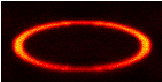
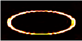
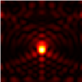
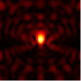
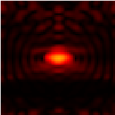
Recently, we proposed to consider additional constraints on the PSF coming from the optical system modeling [21] , [6] . In fact, the confocal microscopy PSF is related to the magnitude of a complex function known as complex valued-amplitude PSF whose shape and support are given in the Fourier domain by the numerical aperture of the optical system [30] , [35] . This latter is known as it is given by the system manufacturer. We incorporate this constraint in the joint PSF and image estimation algorithm [5] by using the Gerchberg-Saxton algorithm (GS) [31] since it allows to alternate constraints in the spatial and frequency domains. Numerical tests on a simulated image of a bead shell are encouraging (cf. figures 2 (a), (b), (c), and (d) presenting $z$-slices of the original image, simulated and reconstructed images). In particular, the added constraint allows to better estimate the PSF shape compared to the previous method [5] (cf. figures 2 (e), (f), and (g)).