Section: New Results

Inverse problems for Poisson-Laplace equations

Participants : Laurent Baratchart, Sylvain Chevillard, Juliette Leblond, Jean-Paul Marmorat, Konstantinos Mavreas, Christos Papageorgakis.

Inverse magnetization issues from planar data

This work is carried out in the framework of the Inria Associate Team Impinge , comprising Cauê Borlina, Eduardo Andrade Lima and Benjamin Weiss from the Earth Sciences department at MIT (Boston, USA) and Douglas Hardin, Edward Saff and Cristobal Villalobos from the Mathematics department at Vanderbilt University (Nashville, USA).

The overall goal of Impinge is to determine magnetic properties of rock samples (e.g. meteorites or stalactites), from weak field measurements close to the sample that can nowadays be obtained using SQUIDs (superconducting quantum interference devices). Depending on the nature of the rock sample, the magnetization distribution can either be considered to lie in a plane or in a parallelepiped of thickness $r$. Some of our results apply to both frameworks (the former appears as a limiting case when $r$ goes to 0), while others concern the 2D case and have no 3-D counterpart yet.

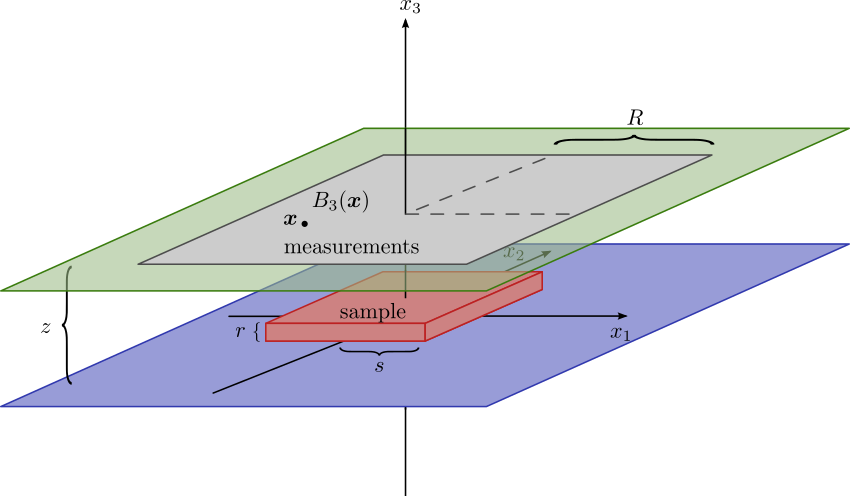
Figure 3 presents a schematic view of the experimental setup: the sample lies on a horizontal plane at height 0 and its support is included in a parallelepiped. The vertical component $B_3$ of the field produced by the sample is measured on points of a horizontal square at height $z$.

We pursued this year our research efforts towards designing algorithms for net moment recovery. The net moment is the integral of the magnetization over its support, and it is a valuable piece of information to physicists which has the advantage of being determined solely by the field: whereas two different magnetizations can generate the same field, the net moment depends only on the field and not on which magnetization produced it. Hence the goal may be described as to build a numerical magnetometer, capable of analyzing data close to the sample. This is in contrast to classical magnetometers which regard the latter as a single dipole, an approximation which is only valid away from the sample and is not suitable to handle weak fields which get quickly blurred by ambient magnetic sources. This research effort was paid in two different, complementary directions.

The first approach consists in using the fact that the integral of $B_3$ against polynomials of order less or equal to 1 on some domains symmetric with respect to the origin provides an estimate of the net moment, asymptotically when $R$ grows large  [34]. This approach was tested this year on real data measured with the SQUID microscope at MIT. Applying directly the formulas on the measured data led to poor results, and we identified this issue as a consequence of electronic noise (drift of the measured field). This noise was impeding the method, especially when $R$ was large, preventing one from getting estimates of the net moment with an error smaller than about $10\%$. By modeling this fairly deterministic drift as an affine function of the space variables, we were able to pretty much cancel out its effect. With this correction, the curve obtained when $R$ varies follows fairly accurately the theoretical asymptotic behavior. We fit this curve with the one corresponding to the theoretical behavior, which allows us to extrapolate its value at infinity, hence giving us an estimate of the net moment. The results on some experimental data (chondrules) are promising. Yet, results on some other data sets are still unsatisfactory and remain to be understood.

The second approach attempts to generalize the previous expansions in the case when $R$ is moderately large. This work is carried out in the thin slab framework, modeling the sample as a rectangle. Last year, we set up a bounded extremal problem (BEP, see Section 3.3.1) consisting in finding the functions ${\phi }_i$ ($i=1,2,3$) such that $|\langle m_i\rangle -\int \int {\phi }_i(x_1,x_2)B_3(x_1,x_2)\mathrm{d}{x}_1\mathrm{d}{x}_2|$ is least possible under the constraint that $\parallel \nabla {\phi }_i{\parallel }_2\le M$, where $M$ is a user-defined parameter. This year, we sharpened our regularity results on the solutions with respect to space variables and the parameters of the problem (e.g., the level of constraint $M$), and considered several resolution schemes. We implemented an algorithm approximately solving for the critical point equation, using a finite elements method. Numerical experiments on synthetic data confirm the validity of the approach with small noise, see [21]. The addition of a synthetic noise, however, has revealed sensitivity to a poor signal / noise ratio, in particular at measurement points close to the edges of the measurement slab where the estimator oscillates heavily. Such oscillations are the price to pay for an estimation procedure which uses data on a measurement set not much bigger than the sample. This is an interesting feature of the method, and further analysis is needed to offset the noise effect. Notice that the work [21] also includes perspectives on minimum $L^2$ regularization for the computation of local moments (which are usually not determined by the field, unlike the net moment).

We started this year to design an alternate procedure to compute a good linear estimator. It consists in expanding it on a family of piecewise affine functions, with a restricted number of pieces. This still needs to be pushed further in connection with the delicate issue of how dense should the grid of data points be in order to reach a prescribed level of precision. On a related topic, we also derived explicit formulas for the adjoint operator $B_3^{*}$ to $B_3$ (in appropriate $L^2$ spaces), when applied to polynomials. This adjoint operator is central to the construction of linear estimators, and these formulas suggest one could work efficiently with polynomial bases. This work is still in progress.

Concerning full inversion of thin samples, after preliminary experiments on regularization with $L^1$ constraints (a heavy trend in linear inverse problems today to favor sparse solutions), we started studying magnetizations modeled by signed measures. A loop decomposition of silent sources was obtained, which makes precise in the 2-D setting the structure theorem of [78]. Moreover, a characterization of equivalent sources having minimal total variation has been obtained when the support of the magnetization is very scattered (purely 1-unrectifiable, which holds in particular for dipolar models) and also for certain magnetizations of geophysical interest like unidirectional ones. Thus, it seems that constraining the total variation to regularize the recovery process is appropriate in some important cases. The theoretical analysis has shown that the optimum is then always sparse, in that it has Hausdorff dimension at most 1. This stems from the real analyticity of operators relating the magnetization to the field, which prevents them from assuming constant level on large sets. An implementation is currently being set up with promising results. Yet, a deeper understanding on how to adjust the parameters of the method is required. This topic is studied in collaboration with D. Hardin and C. Villalobos from Vanderbilt University.

Besides, we considered a simplified 2-D setup for magnetizations and magnetic potentials (of which the magnetic field is the gradient). When both the sample and the measurement set are parallel intervals, some best approximation issues related to inverse recovery and relevant BEP problems in Hardy classes of holomorphic functions (see Section 3.3.1) were solved in [19]. Note that, in the present case, the criterion no longer acts on the boundary of the holomorphy domain (namely, the upper half-plane), but on a strict subset thereof, while the constraint acts on the support of the approximating function. Both involve real parts of functions in the Hilbert Hardy space of the upper half-plane. This is joint work with D. Ponomarev (see Section 7.5.1). Some extensions are the subject of ongoing work with E. Pozzi (Department of Mathematics and Statistics, St Louis Univ., St Louis, Missouri, USA). They concern more precise approximation criteria, and the development of resolution schemes using the Fourier basis. Meanwhile, BEP in Bergman classes of analytic or generalized analytic functions are under being studied with B. Delgado Lopez (see Sections 3.2, 7.5.1).

For magnetizations supported in a volume $\Omega$ with boundary $\partial \Omega$, there is a greater variety of silent sources, since they have much more space to live in. Now, to each magnetization $m$ supported in $\Omega$ there is a unique magnetization supported on $\partial \Omega$ (the balayage of $m$) and producing the same field outside $\Omega$. Thus, describing silent sources supported on $\partial \Omega$ is a way to factor out some of the complexity of the situation. When $m$ is located in the plane, the Hardy-Hodge decomposition introduced in [38] (see Section 3.3.1) was used there to characterize all silent magnetizations from above (resp.below) as being those having no harmonic gradient from below (rep. above) in their decomposition. When $m$ is supported on a compact surface, a similar decomposition exists for ${ℝ}^3$-valued vector fields on $\partial \Omega$, (see Section 5.4), that allows to characterize all magnetizations on $\partial \Omega$ which are silent from outside as being those whose harmonic components satisfy a certain spectral relation for the double layer potential on $\partial \Omega$. The analysis and the algorithmic use of that equation for recovery or moment estimation remain to be worked out.

Other types of inverse magnetization problems can be tackled using such techniques, in particular global Geomagnetic issues which arise in spherical geometry. This year, in collaboration with C. Gerhards from the University of Vienna (Austria), we developed a method to separate the crustal component of the Earth's magnetic field from its core component, if an estimate of the field is known on a subregion of the globe [23] . This assumption is not unrealistic: parts of Australia and of northern Europe are considered as fairly well understood from the magnetostatic view point. We look forward to test the algorithm against real data, in collaboration with Geophysicists

Inverse magnetization issues from sparse cylindrical data

The team Apics is a partner of the ANR project MagLune on Lunar magnetism, headed by the Geophysics and Planetology Department of Cerege, CNRS, Aix-en-Provence (see Section 7.2.2). Recent studies let geoscientists think that the Moon used to have a magnetic dynamo for a while. However, the exact process that triggered and fed this dynamo is still not understood, much less why it stopped. The overall goal of the project is to devise models to explain how this dynamo phenomenon was possible on the Moon.

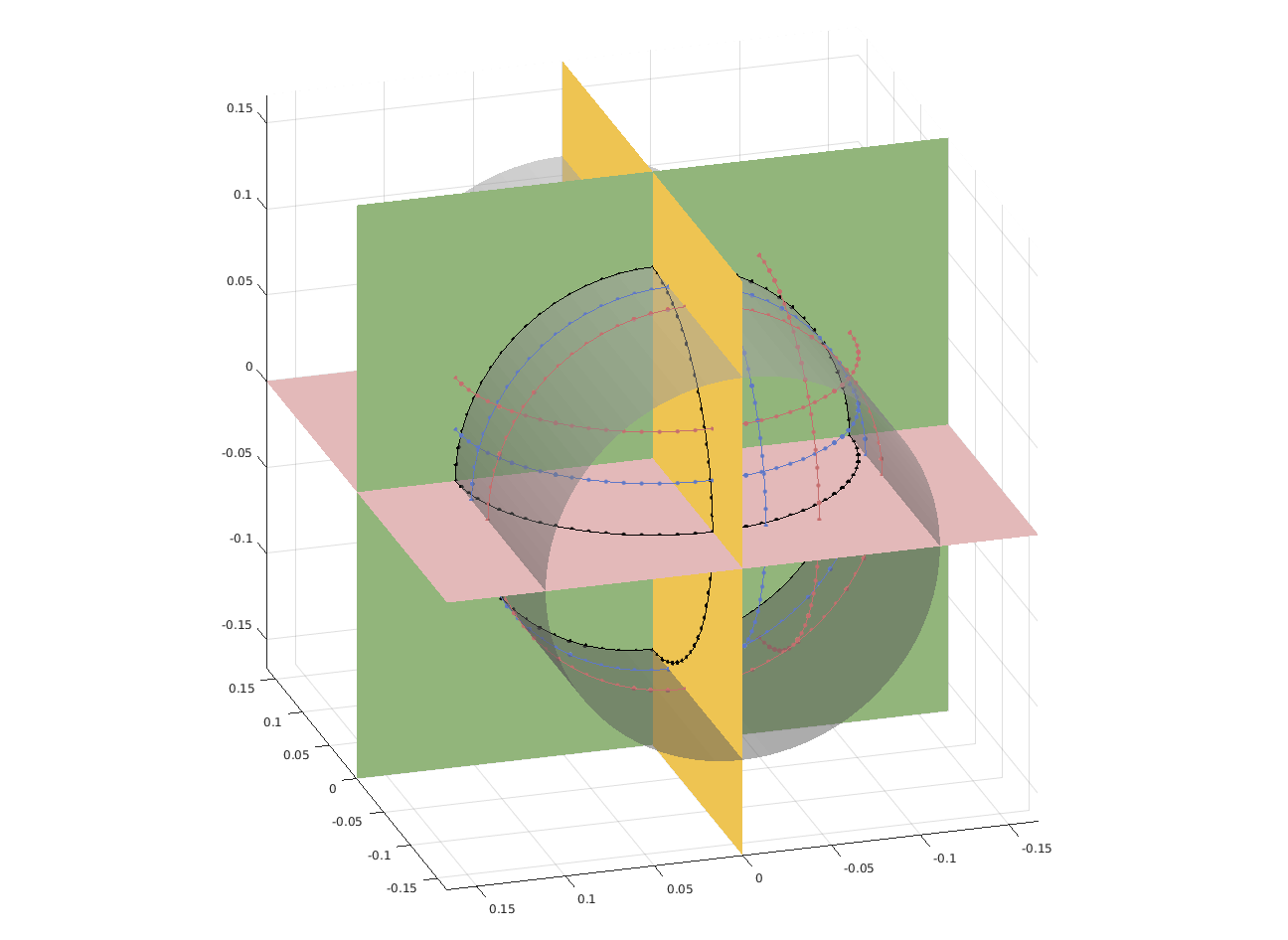
The geophysicists from Cerege went a couple of times to NASA to perform measurements on a few hundreds of samples brought back from the Moon by Apollo missions. The samples are kept inside bags with a protective atmosphere, and geophysicists are not allowed to open the bags, nor to take out samples from NASA facilities. Moreover, the process must be carried out efficiently as a fee is due to NASA by the time when handling these moon samples. Therefore, measurements were performed with some specific magnetometer designed by our colleagues from Cerege. This device measures the components of the magnetic field produced by the sample, at some discrete set of points located on circles belonging to three cylinders (see Figure 4). The objective of Apics is to enhance the numerical efficiency of post-processing data obtained with this magnetometer.

This year, we continued the approach taken in previous years. Under the hypothesis that the field can be well explained by a single magnetic pointwise dipole, and using ideas similar to those underlying the FindSources3D tool (see Sections 3.4.2 and 5.1.3), we try to recover the position and the moment of the dipole using the available measurements.

In a given cylinder, using the associated cylindrical system of coordinates, recovering the position of the dipole boils down to determine its height $z$, its radial distance $\rho$ and its azimuth $\phi$. In principle, the rational approximation technique that we are using returns, for the circle of measurements at height $h$, the unique complex pole ${\xi }_h$ of order five belonging to the corresponding normalized disk of some rational function. From this pole, the complex number $u_h={\xi }_h+\frac{1}{\overline{{\xi }_h}}=\frac{1+{\rho }^2+{(h-z)}^2}{\rho }{e}^{i\phi }$ can be estimated. In practice, due to the fact that the field is not truly generated by a single dipole, and also because of noise in the measurements and numerical errors in the rational approximation step, only an approximation of $u_h$ is computed. The question is then to reliably combine the information provided by all circles of measurements, in order to recover $z$, $\rho$ and $\phi$. The azimuth is fairly easy to obtain: we can estimate it, e.g., by taking the mean value of the argument of ${\xi }_h$, for all $h$ for which we have a measurement circle, possibly excluding one of them when the provided estimate seems to be clearly different from the others. As regards the reconstruction of $\rho$ and $z$, we designed this year two new strategies.

The first strategy consists in observing that $\rho |u_h|=1+{\rho }^2+h^2-2hz+z^2$, whence doing the difference with the same equation obtained at height $h^{\text{'}}$: $\rho \left(\right|u_h|-|u_{h^{\text{'}}}\left|\right)=(h^2-h^{\text{'}2})-2(h-h^{\text{'}})z$. This provides a linear relation between the unknowns $\rho$ and $z$. Three measurement circles provide us with two independent relations and are in principle enough to recover $\rho$ and $z$. Numerical experiments showed that this recovery strategy is unsatisfactory: it is fairly sensitive to approximation errors on the estimates $|u_h|$ and $|u_{h^{\text{'}}}|$, hence the estimation procedure is unstable. However, it might become more robust if data were available on more than three circles per cylinder. Exploring this idea is an on-going piece of work. If successful, it will suggest an easy modification of the magnetometer of Cerege for future measurements campaigns.

The second strategy directly uses the pole ${\xi }_h$ instead of $u_h$, hence avoiding numerical steps that are possible sources of errors. It consists in observing that $|{\xi }_h|$ is maximal, with respect to $h$, when $h=z$ and it is then equal to $\rho e^{i\phi }$. A rough estimate of $\rho$ is hence given by the maximal value of $|{\xi }_h|$ among the three values of $h$ available for each cylinder. The position of the dipolar source is then estimated by combining the estimates of $\rho$ and $\phi$ obtained on all three cylinders. The moment is then computed from this estimated position, solving a linear system by least-squares techniques. Although not sophisticated, this method gave promising results on synthetic examples, with more or less noise, see the submitted work [25]. This is still on-going work which constitutes the main topic of the PhD thesis of K. Mavreas.

Inverse problems in medical imaging

This work is conducted in collaboration with Maureen Clerc and Théo Papadopoulo, from the team Athena (Inria Sophia).

In 3-D, functional or clinically active regions in the cortex are often modeled by pointwise sources that have to be localized from measurements, taken by electrodes on the scalp, of an electrical potential satisfying a Laplace equation (EEG, electroencephalography). In the works [6], [43] on the behavior of poles in best rational approximants of fixed degree to functions with branch points, it was shown how to proceed via best rational approximation on a sequence of 2-D disks cut along the inner sphere, for the case where there are finitely many sources (see Section 4.3).

In this connection, a dedicated software FindSources3D (FS3D, see Section 3.4.2) is being developed, in collaboration with the Inria team Athena and the CMA - Mines ParisTech. In addition to the modular and ergonomic platform version of FS3D, a new (Matlab) version of the software that automatically performs the estimation of the quantity of sources is being built. It uses an alignment criterion in addition to other clustering tests for the selection. It appears that, in the rational approximation step, multiple poles possess a nice behavior with respect to branched singularities. This is due to the very physical assumptions on the model (for EEG data that correspond to measurements of the electrical potential, one should consider triple poles; for (magnetic) field data however, like in Section 5.1.2 or from MEG – magneto-encephalography – data, one should consider poles of order five). Though numerically observed in [7], there is no mathematical justification so far why multiple poles generate such strong accumulation of the poles of the approximants. This intriguing property, however, is definitely helping source recovery. It is used in order to automatically estimate the “most plausible” number of sources (numerically: up to 3, at the moment). Last but not least, the version of the software currently under development takes as inputs actual EEG measurements, like time signals, and performs a suitable singular value decomposition in order to separate independent sources.

Magnetic data from MEG recently became available along with EEG data, by our medical partners at the hospital la Timone; indeed, it is now possible to use simultaneously both measurement devices, in order to measure both the electrical potential and a component of the magnetic fields. This should enhance the accuracy of our source recovery algorithms. We will add the treatment of MEG data as another functionality of the software FS3D.

In connection with these and other brain exploration modalities like electrical impedance tomography (EIT), we are now studying conductivity estimation problems. This is the topic of the PhD research work of C. Papageorgakis (co-advised with the Inria team Athena and BESA GmbH, see Section 6.1.2). In layered models, it concerns the estimation of the conductivity of the skull (an intermediate layer). First, the conductivity of the skull can differ from one individual to another, or for the same person, along the time, and is much smaller than those of the surrounding layers (the brain and the scalp). A preliminary issue in this direction was to estimate a single-valued skull conductivity from one EEG recording. Existence, uniqueness, stability properties and a recovery scheme for this conductivity value were established in the spherical setting when the sources are known, see [10]. When the sources are unknown, we must look for additional data (additional clinical and/or functional EEG, EIT, ...) that could be incorporated in order to recover both the sources locations and the skull conductivity. Second, while the skull essentially consists of a hard bone part, which may be assumed to have constant electrical conductivity, it also contains spongy bone compartments. These two distinct components of the skull actually possess quite different conductivities. The influence of the second on the overall model is also studied in [10], together with a numerical process allowing to estimate the hard bone conductivity value together with a dipolar source, in realistic geometries.

We also began to consider the inverse problem of recovering the parameters of a skin tumor from thermal measurements, in a 2-D model that takes the form of a static Schrödinger equation. This is joint work with F. Ferranti (IMT Atlantique, Microwave Department) and the topic of the internship of G. Dervaux, see Section 7.5.1.