Section: Overall Objectives

General scope and motivations

Nonsmooth dynamics concerns the study of the time evolution of systems that are not smooth in the mathematical sense, i.e., systems that are characterized by a lack of differentiability, either of the mappings in their formulations, or of their solutions with respect to time. The class of nonsmooth dynamical systems recovers a large variety of dynamical systems that arise in many applications. The term “nonsmooth”, as the term “nonlinear”, does not precisely define the scope of the systems we are interested in but, and most importantly, they are characterized by the mathematical and numerical properties that they share. To give more insight of what are nonsmooth dynamical systems, we give in the sequel a very brief introduction of their salient features. For more details, we refer to [1], [2] [61], [78], [94], [63], [39].

A flavor of nonsmooth dynamical systems

As a first illustration, let us consider a linear finite-dimensional system described by its state $x\left(t\right)\in {IR}^n$ over a time-interval $t\in [0,T]$:

subjected to a set of $m$ inequality (unilateral) constraints:

If the constraints are physical constraints, a standard modeling approach is to augment the dynamics in (1) by an input vector $\lambda \left(t\right)\in {IR}^m$ that plays the role of a Lagrange multiplier vector. The multiplier restricts the trajectory of the system in order to respect the constraints. Furthermore, as in the continuous optimization theory, the multiplier must be signed and must vanish if the constraint is not active. This is usually formulated as a complementarity condition:

which models the one-sided effect of the inequality constraints. The notation $y\ge 0$ holds component–wise and $y\perp \lambda$ means $y^T\lambda =0$. All together we end up with a Linear Complementarity System (LCS) of the form,

where $B\in {IR}^{n\times m}$ is the matrix that models the input generated by the constraints. In a more general way, the constraints may also involve the Lagrange multiplier,

leading to a general definition of LCS as

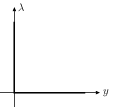
The complementarity condition, illustrated in Figure 1 is the archetype of a nonsmooth graph that we extensively use in nonsmooth dynamics. The mapping $y\mapsto \lambda$ is a multi-valued (set-valued) mapping, that is nonsmooth at the origin. It has a lot of interesting mathematical properties and reformulations that come mainly from convex analysis and variational inequality theory. Let us introduce the indicator function of ${IR}_{+}$ as

This function is convex, proper and can be sub-differentiated  [67]. The definition of the subdifferential of a convex function $f:{IR}^m\to IR$ is defined as:

A basic result of convex analysis reads as

that gives a first functional meaning to the set-valued mapping $y\mapsto \lambda$. Another interpretation of $\partial {\Psi }_{{IR}_{+}}$ is based on the normal cone to a closed and nonempty convex set $C$:

It is easy to check that $\partial {\Psi }_{{IR}_{+}}=N_{{IR}_{+}}\left(x\right)$ and it follows that

Finally, the definition of the normal cone yields a variational inequality:

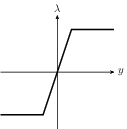
The relations (11) and (12) allow one to formulate the complementarity system with $D=0$ as a differential inclusion based on a normal cone (see (15)) or as a differential variational inequality. By extending the definition to other types of convex functions, possibly nonsmooth, and using more general variational inequalities, the same framework applies to the nonsmooth laws depicted in Figure 2 that includes the case of piecewise smooth systems.

The mathematical concept of solutions depends strongly on the nature of the matrix quadruplet $(A,B,C,D)$ in (6). If $D$ is a positive definite matrix (or a $P$-matrix), the Linear Complementarity problem

admits a unique solution $\lambda \left(x\right)$ which is a Lipschitz continuous mapping. It follows that the Ordinary Differential Equation (ODE)

is a standard ODE with a Lipschitz right-hand side with a $C^1$ solution for the initial value problem. If $D=0$, the system can be written as a differential inclusion in a normal cone as

that admits a solution that is absolutely continuous if $CB$ is a definite positive matrix and the initial condition satisfies the constraints. The time derivative $\dot{x}\left(t\right)$ and the multiplier $\lambda \left(t\right)$ may have jumps and are generally considered as functions of bounded variations. If $CB=0$, the order of nonsmoothness increases and the Lagrange multiplier may contain Dirac atoms and must be considered as a measure. Higher–order index, or higher relative degree systems yield solutions in terms of distributions and derivatives of distributions  [33].

A lot of variants can be derived from the basic form of linear complementarity systems, by changing the form of the dynamics including nonlinear terms or by changing the complementarity relation by other multivalued maps. In particular the nonnegative orthant may be replaced by any convex closed cone $K\subset {IR}^m$ leading to complementarity over cones

where $K^{☆}$ its dual cone given by

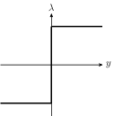
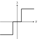
In Figure 2, we illustrate some other basic maps that can used for defining the relation between $\lambda$ and $y$. The saturation map, depicted in Figure 2(a) is a single valued continuous function which is an archetype of piece-wise smooth map. In Figure 2(b), the relay multi-function is illustrated. If the upper and the lower limits of $\lambda$ are respectively equal to 1 and $-1$, we obtain the multivalued sign function defined as

Using again convex analysis, the multivalued sign function may be formulated as an inclusion into a normal cone as

More generally, any system of the type,

can reformulated in terms of the following set-valued system

The system (21) appears in a lot of applications; among them, we can cite the sliding mode control, electrical circuits with relay and Zener diodes  [29], or mechanical systems with friction  [31].

Though this class of systems seems to be rather specific, it includes as well more general dynamical systems such as piecewise smooth systems and discontinuous ordinary differential equations. Indeed, the system (20) for scalars $y$ and $\lambda$ can be viewed as a discontinuous differential equation:

One of the most well-known mathematical framework to deal with such systems is the Filippov theory  [61] that embed the discontinuous differential equations into a differential inclusion. In the case of a single discontinuity surface given in our example by $S=\{x\mid Cx+c=0\}$, the Filippov differential inclusion based on the convex hull of the vector fields in the neighborhood of $S$ is equivalent to the use of the multivalued sign function in (20). Conversely, as it has been shown in [37], a piecewise smooth system can be formulated as a nonsmooth system based on products of multivalued sign functions.

Nonsmooth Dynamical systems in the large

Generally, the nonsmooth dynamical systems we propose to study mainly concern systems that possess the following features:

1. A nonsmooth formulation of the constitutive/behavioral laws that define the system. Examples of nonsmooth formulations are piecewise smooth functions, multi–valued functions, inequality constraints, yielding various definitions of dynamical systems such as piecewise smooth systems, discontinuous ordinary differential equations, complementarity systems, projected dynamical systems, evolution or differential variational inequalities and differential inclusions (into normal cones). Fundamental mathematical tools come from convex analysis  [87], [68], [67], complementarity theory  [57], and variational inequalities theory  [60].

2. A concept of solutions that does not require continuously differentiable functions of time. For instance, absolutely continuous, Lipschitz continuous functions or functions of local bounded variation are the basis for solution concepts. Measures or distributions are also solutions of interest for differential inclusions or evolution variational inequalities.

Nonsmooth systems versus hybrid systems

The nonsmooth dynamical systems we are dealing with, have a nonempty intersection with hybrid systems and cyber-physical systems, as it is briefly discussed in Sect. 3.2.4. Like in hybrid systems, nonsmooth dynamical systems define continuous–time dynamics that can be identified to modes separated by guards, defined by the constraints. However, the strong mathematical structure of nonsmooth dynamical systems allows us to state results on the following points:

1. Mathematical concept of solutions: well-posedness (existence, and possibly, uniqueness properties, (dis)continuous dependence on initial conditions).

2. Dynamical systems theoretic properties: existence of invariants (equilibria, limit cycles, periodic solutions,...) and their stability, existence of oscillations, periodic and quasi-periodic solutions and propagation of waves.

3. Control theoretic properties: passivity, controllability, observability, stabilization, robustness.

These latter properties, that are common for smooth nonlinear dynamical systems, distinguish the nonsmooth dynamical systems from the very general definition of hybrid or cyber-physical systems  [42], [66]. Indeed, it is difficult to give a precise mathematical concept of solutions for hybrid systems since the general definition of hybrid automata is usually too loose.

Numerical methods for nonsmooth dynamical systems

To conclude this brief exposition of nonsmooth dynamical systems, let us recall an important fact related to numerical methods. Beyond their intrinsic mathematical interest, and the fact that they model real physical systems, using nonsmooth dynamical systems as a model is interesting, because it exists a large set of robust and efficient numerical techniques to simulate them. Without entering into deeper details, let us give two examples of these techniques:

• Numerical time integration methods: convergence, efficiency (order of consistency, stability, symplectic properties). For the nonsmooth dynamical systems described above, there exist event–capturing time–stepping schemes with strong mathematical results. These schemes have the ability to numerically integrate the initial value problem without performing an event location, but by capturing the event within a time step. We call an event, or a transition, every change into the index set of the active constraints in the complementarity formulation or in the normal cone inclusion. Hence these schemes are able to simulate systems with a huge number of transitions or even worth finite accumulation of events (Zeno behavior). Furthermore, the schemes are not suffering from the weaknesses of the standard schemes based on a regularization (smoothing) of the multi-valued mapping resulting in stiff ordinary differential equations. For the time–integration of the initial value problem (IVP), or Cauchy problem, a lot of improvements of the standard time–stepping schemes for nonsmooth dynamics (Moreau–Jean time-stepping scheme) have been proposed in the last decade, in terms of accuracy and dissipation properties  [26], [27], [88], [89], [28], [56], [52], [90], [54]. An important part of these schemes has been developed by members of the BIPOP team and has been implemented in the Siconos software (see Sect. 5.1).

• Numerical solution procedure for the time–discretized problem, mainly through well-identified problems studied in the optimization and mathematical programming community. Another very interesting feature is the fact that the discretized problem that we have to solve at each time–step is generally a well-known problem in optimization. For instance, for LCSs, we have to solve a linear complementarity problem  [57] for which there exist efficient solvers in the literature. Comparing to the brute force algorithm with exponential complexity that consists in enumerating all the possible modes, the algorithms for linear complementarity problem have polynomial complexity when the problem is monotone.

In the Axis 2 of the research program (see Sect. 3.3), we propose to perform new research on the geometric time-integration schemes of nonsmooth dynamical systems, to develop new integration schemes for Boundary Value Problem (BVP), and to work on specific methods for two time-discretized problems: the Mathematical Program with Equilibrium Constraints (MPEC) for optimal control and Second Order Cone Complementarity Problems (SOCCP) for discrete frictional contact systems.