Section: New Results

Inverse problems for Poisson-Laplace equations

Participants : Laurent Baratchart, Sylvain Chevillard, Juliette Leblond, Konstantinos Mavreas, Christos Papageorgakis, Dmitry Ponomarev.

This section is concerned with inverse problems for 3-D Poisson-Laplace equations, among which source recovery issues. Though the geometrical settings differ in Sections 5.1.1 and 5.1.5, the characterization of silent sources (those giving rise to a vanishing field) is one common problem to both cases. The latter has been resolved in the magnetization setup for thin slabs [36]. The case of volumetric distribution is currently being investigated, starting with magnetization distributions on closed surfaces to which the general volumetric case can be reduced by balayage.

Inverse magnetization issues in the thin-plate framework

This work is carried out in the framework of the Inria Associate Team Impinge , comprising Eduardo Andrade Lima and Benjamin Weiss from the Earth Sciences department at MIT (Boston, USA) and Douglas Hardin, Michael Northington, Edward Saff and Cristobal Villalobos from the Mathematics department at Vanderbilt University (Nashville, USA).

The overall goal of Impinge is to determine magnetic properties of rock samples (e.g. meteorites or stalactites) from weak field measurements close to the sample that can nowadays be obtained using SQUIDs (superconducting quantum interference devices). During previous years, we always considered the case when the rock is cut into slabs so thin that the magnetization distribution could be considered to lie in a plane. This year, we started considering the situation where the thickness $r$ of the sample cannot be ignored. The thin-slab case thus appears as a limiting case when $r$ goes to 0.

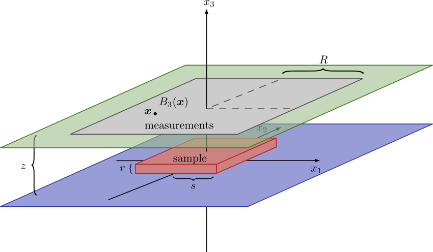
Figure 3 presents a schematic view of the experimental setup: the sample lies on a horizontal plane at height 0 and its support is included in a parallelepiped. The vertical component $B_3$ of the field produced by the sample is measured on points of a horizontal square at height $z$.

We focused on net moment recovery, the net moment of a magnetization being given by its mean value on the sample. The net moment is a valuable piece of information to Physicists and has the advantage of being well-defined: whereas two different magnetizations can generate the same field, the net moment depends only on the field and not on the magnetization itself. Hence the goal may be described as building a numerical magnetometer, capable of analyzing data close to the sample. This is in contrast to classical magnetometers which regard the latter as a single dipole, an approximation which is only valid away from the sample and is not suitable to handle weak fields which get quickly blurred by ambient magnetic sources. This research effort was paid in two different, complementary directions.

The first approach consists in computing asymptotic expansions of the integrals $\int \int B_3(x_1,x_2,z)\mathrm{d}{x}_1\mathrm{d}{x}_2$, $\int \int x_1{B}_3(x_1,x_2,z)\mathrm{d}{x}_1\mathrm{d}{x}_2$ and $\int \int x_2{B}_3(x_1,x_2,z)\mathrm{d}{x}_1\mathrm{d}{x}_2$, on several domains (namely, the 2-D balls of radius $R$ for the 1, 2 and $\infty$ norm, that are squares, disks, diamonds), in terms of the moments of first and higher order of the magnetization $m$. Last year, we obtained formulas valid only under the thin-slab hypothesis. This year, we extended the results to the case of a volumetric magnetization. We posted a preprint [22] with these results on HAL, and our partners at MIT are currently conducting practical experiments with the SQUID to illustrate the method, before submitting it to some journal. In parallel, Fourier based techniques designed by reformulating the problem with the help of the Kelvin transform also furnish an asymptotic expansion of the net moment involving, at the first order, the above-mentioned integrals computed on disks of large radius. The computations are quite involved but allow to obtain higher-order terms. This constitutes Part III of D. Ponomarev's PhD work [11], defended this year.

The second approach attempts to generalize the previous expansions. The initial question is: given measurements of $B_3$, find a function $\phi (x_1,x_2)$ such that $\int \int \phi (x_1,x_2)B_3(x_1,x_2)\mathrm{d}{x}_1\mathrm{d}{x}_2$ is best possible an estimate of the net moment components $\langle m_i\rangle$ ($i=1,2,3$), in some appropriate sense. This problem has no solution really because, for any $ϵ>0$, there exists a function ${\phi }_{ϵ}$ allowing to estimate the moment with an error bounded by $ϵ$. We proved that, when $ϵ$ tends to zero, the norm of the function ${\phi }_{ϵ}$ tends to infinity, which hinders an accurate numerical computation of the integral since $B_3$ is only known on a discrete grid of points. We therefore expressed the problem as a bounded extremal problem (see Section 3.3.1): to find the best ${\phi }_{ϵ}$ (with the smallest possible error value $ϵ$) under the constraint that $\parallel \nabla {\phi }_{ϵ}{\parallel }_2\le M$. Here, $M$ is a user-defined parameter. We improved on the iterative algorithm devised last year and completed the theoretical justification of its convergence. Basic properties of the operators involved, which are necessary to carry out the procedure, have been derived in [21], along with perspectives on minimum $L^2$ regularization for the computation of local moments (which are usually not determined by the field, unlike the net moment).

We also performed preliminary numerical experiments which are very encouraging, but still need to be pushed further in connection with the delicate issue of how dense should the grid of data points be in order to reach a prescribed level of precision. An article on this topic is in preparation.

In this connection, the PhD thesis of D. Ponomarev's [11], Part II, contains a study of the 2D spectral problem for the truncated Poisson operator in planar geometry. This is a simplified (i.e. 2-D) setup for the relation between the magnetization and the magnetic potential, of which the magnetic field is the gradient. It is relevant because, by the familiar Courant min-max principle, the eigenvectors of the magnetization-to-field operator produce in principle an efficient basis to expand a given magnetization in short series. Describing these eigenvectors is a long-standing problem. Asymptotic formulas as the measurement height gets small with respect to the size of the sample have been obtained, both for dominant eigenvalues and eigenvectors, through connections with other spectral problems. In fact, asymptotic reductions for large and small values of the main parameters (distance $h$ from the measurement plane to the sample support and sample support size), yield approximate solutions by means of simpler integral equations and ODEs.

Inverse magnetization issues from sparse spherical data

The team Apics is a partner of the ANR project MagLune on Lunar magnetism, headed by the Geophysics and Planetology Department of Cerege, CNRS, Aix-en-Provence (see Section 7.2.2). Recent studies let geoscientists to think that the Moon used to have a magnetic dynamo for a while, yet the exact process that triggered and fed this dynamo is still not understood, much less why it stopped. The overall goal of the project is to devise models to explain how this dynamo phenomenon was possible on the Moon.

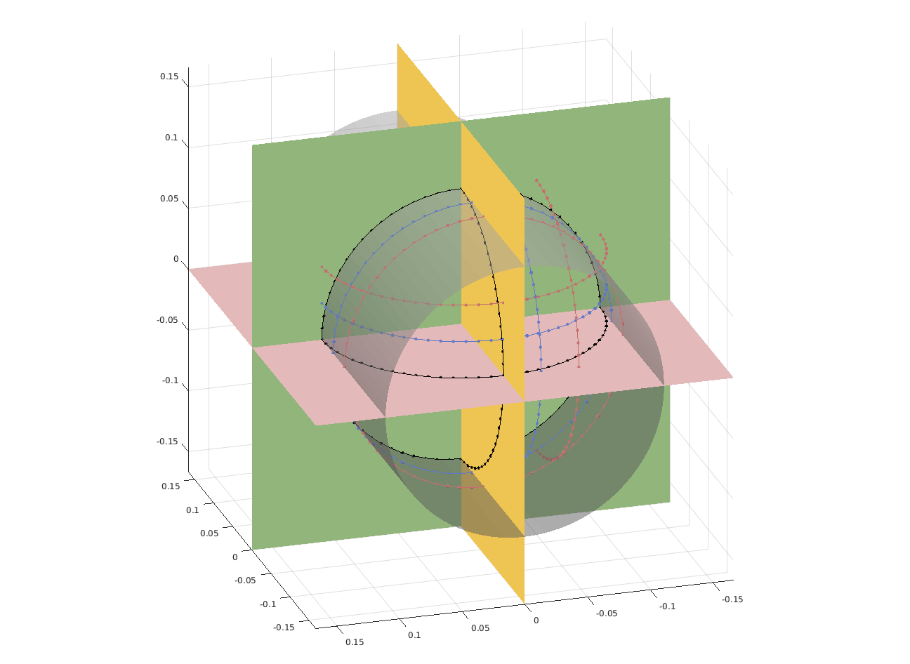
The geophysicists from Cerege went this year to NASA to perform measurements on a few hundreds of samples brought back from the Moon by Apollo missions. The samples are kept inside bags with a protective atmosphere, and geophysicists are not allowed to open the bags, nor to take out samples from NASA facilities. Moreover, the process must be carried out efficiently as a fee is due to NASA by the time when handling these moon samples. Therefore, measurements were performed with some specific magnetometer designed by our colleagues from Cerege. This device measures the components of the magnetic field produced by the sample, at some discrete set of points located on circles belonging to three cylinders (see Figure 4). The objective of Apics is to enhance the numerical efficiency of post-processing data obtained with this magnetometer.

This year, we continued the approach initiated in 2015 during K. Mavreas' internship: under the hypothesis that the field can be well explained by a single magnetic dipole, and using ideas similar to those underlying the FindSources3D tool (see Sections 3.4.2 and 5.1.5), we try to recover the position and moment of the dipole. The rational approximation technique that we are using gives, for each circle of measurements, a partial information about the position of the dipole. These partial informations obtained on all nine circles must then be combined in order to recover the exact position. Theoretically speaking, the nine partial informations are redundant and the position could be obtained by several equivalent techniques. But in practice, due to the fact that the field is not truly generated by a single dipole, and also because of noise in the measurements and numerical errors in the rational approximation step, all methods do not show the same reliability when combining the partial results. We studied several approaches, testing them on synthetic examples, with more or less noise, in order to propose a good heuristic for the reconstruction of the position. This is still on-going work.

Surface distributed magnetizations and vector fields decomposition

This is a joint work with Pei Dang and Tao Qian from the University of Macao.

Silent magnetizations in the thin plate case were characterized in [36] using a decomposition of ${ℝ}^3$-valued vector fields defined on ${ℝ}^2\sim {ℝ}^2\times \left\{0\right\}\subset {ℝ}^3$. More precisely, in rather general smoothness classes (involving all distributions with compact support), such a vector field is the sum of the traces on ${ℝ}^2$ of a harmonic gradient in the upper half space, a harmonic gradient in the lower half space, and of a tangential divergence-free vector field. This year the corresponding decomposition has been obtained in $L^p$-classes on closed surfaces, where $1<p<\infty$ if the surface is smooth but $p$ has to be restricted around the value 2 if the surface is only Lipschitz smooth. The proof uses elliptic regularity theory, some Hodge theory and Clifford analysis.

In the case where the curvature is constant (i.e. for spheres and planes), one recovers using the previous result that silent distribution have no inner harmonic gradient component, whereas in the case of more general surfaces one finds they have to satisfy a spectral equation for the double layer potential. This also furnishes a characterization of volumetric silent distributions by saying that their balayage to the boundary of the volume (which is a closed surface) is silent. An article is being written on this topic.

Decomposition of the geomagnetic field

This is a joint work with Christian Gerhards from the University of Vienna.

The techniques based on solving bounded extremal problems, set forth in Section 5.1.1 to estimate the net moment of a planar magnetization, may be used to approach the problem of decomposing the magnetic field of the Earth into its crustal and core components, when adapted to a spherical geometry.

Indeed, in geomagnetism it is of interest to separate the Earth's core magnetic field from the crustal magnetic field. However, satellite measurements can only sense the superposition of the two contributions. In practice, the measured magnetic field is expanded in terms of spherical harmonics and a separation into crust and core contribution is done empirically by a sharp cutoff in the spectral domain. Under the assumption that the crustal magnetic field is supported on a strict subset of the Earth's surface, which is nearly verified as some regions on the globe are only very weakly magnetic, one can state an extremal problem to find a linear form yielding an arbitrary coefficient of the expansion in spherical harmonics on the crustal field, while being nearly zero on the core contribution. An article is being prepared to report on this research.

Inverse problems in medical imaging

This work is conducted in collaboration with Jean-Paul Marmorat and Nicolas Schnitzler, together with Maureen Clerc and Théo Papadopoulo from the Athena EPI.

In 3-D, functional or clinically active regions in the cortex are often modeled by pointwise sources that have to be localized from measurements, taken by electrodes on the scalp, of an electrical potential satisfying a Laplace equation (EEG, electroencephalography). In the works [6], [41] on the behavior of poles in best rational approximants of fixed degree to functions with branch points, it was shown how to proceed via best rational approximation on a sequence of 2-D disks cut along the inner sphere, for the case where there are finitely many sources (see Section 4.3).

In this connection, a dedicated software FindSources3D (see Section 3.4.2) is being developed, in collaboration with the team Athena and the CMA. In addition to the modular and ergonomic platform version of FindSources3D, a new (Matlab) version of the software that automatically performs the estimation of the quantity of sources is being built. It uses an alignment criterion in addition to other clustering tests for the selection. It appears that, in the rational approximation step, multiple poles possess a nice behavior with respect to branched singularities. This is due to the very physical assumptions on the model (for EEG data, one should consider triple poles). Though numerically observed in [7], there is no mathematical justification so far why multiple poles generate such strong accumulation of the poles of the approximants. This intriguing property, however, is definitely helping source recovery. It is used in order to automatically estimate the “most plausible” number of sources (numerically: up to 3, at the moment). Last but not least, this new version may take as inputs actual EEG measurements, like time signals, and performs a suitable singular value decomposition in order to separate independent sources.

In connection with these and other brain exploration modalities like electrical impedance tomography (EIT), we are now studying conductivity estimation problems. This is the topic of the PhD research work of C. Papageorgakis (co-advised with the Athena project-team and BESA GmbH). In layered models, it concerns the estimation of the conductivity of the skull (intermediate layer). Indeed, the skull was assumed until now to have a given isotropic constant conductivity, whose value can differ from one individual to another. A preliminary issue in this direction is: can we uniquely recover and estimate a single-valued skull conductivity from one EEG recording? This has been established in the spherical setting when the sources are known, see [14]. Situations where sources are only partially known and the geometry is more realistic than a sphere are currently under study. When the sources are unknown, we should look for more data (additional clinical and/or functional EEG, EIT, ...) that could be incorporated in order to recover both the sources locations and the skull conductivity. Furthermore, while the skull essentially consists of a hard bone part, which may be assumed to have constant electrical conductivity, it also contains spongy bone compartments. These two distinct components of the skull possess quite different conductivities. The influence of the second on the overall model is currently being studied.