Section: Scientific Foundations

Adaptive torsion-angle mechanics

In many situations, it is preferable to represent molecular systems as articulated bodies, and perform so-called torsion-angle mechanics. This may be to allow for larger time step sizes in a simulation, or because the user wants to focus to e.g. protein backbone deformations.

We have also developed an adaptive mechanics algorithm in the case of torsion-angle representations. In this case, a molecular system is recursively defined as the assembly of two molecular systems connected by a joint (when connecting two subassemblies which belong to the same molecule) or, more generally, by a rigid body transform (to assemble several molecules).

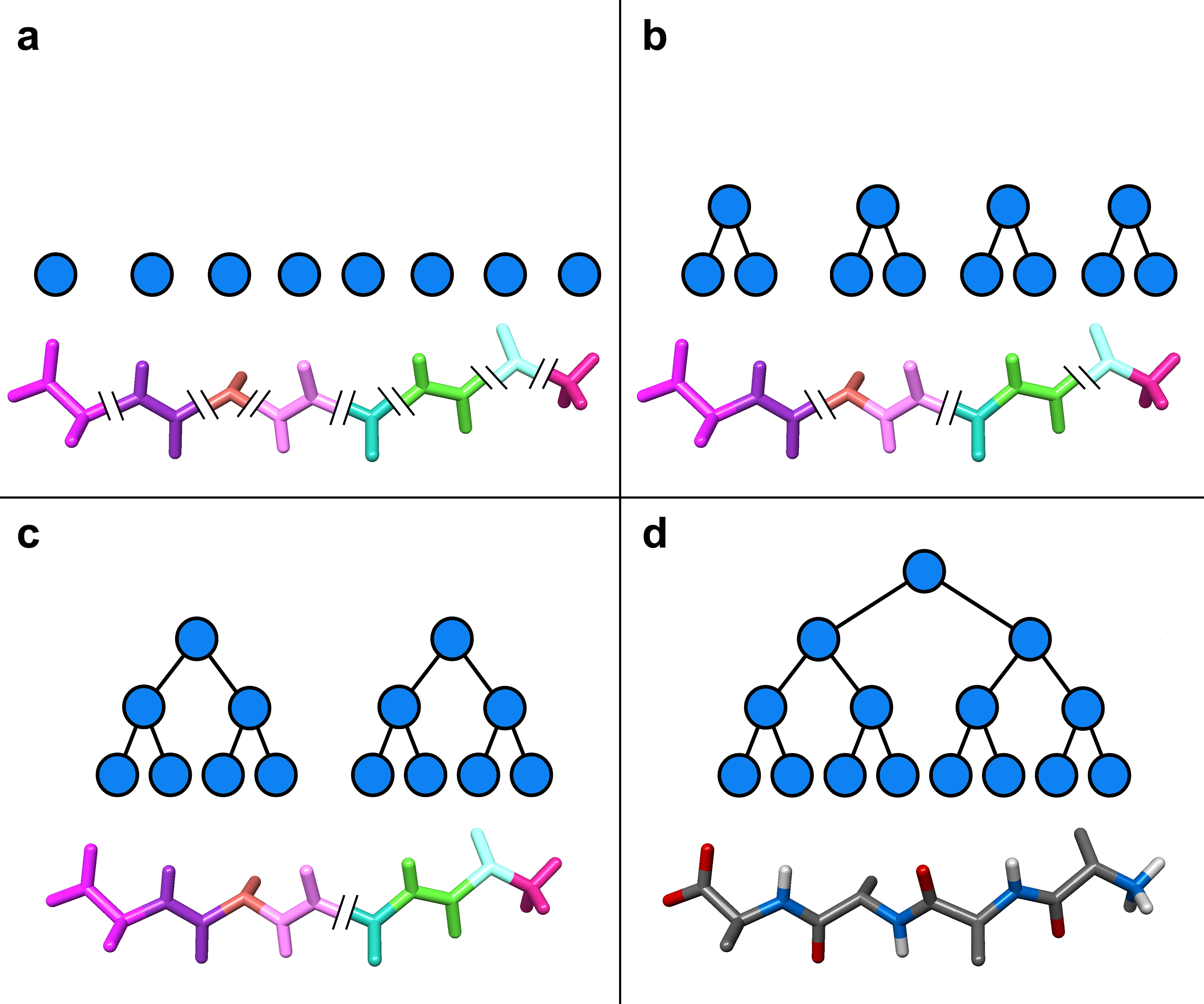
As in the Cartesian mechanics case, the complete molecular system is thus also represented by a binary tree, in which leaves are rigid bodies (a rigid body can be a single atom), internal nodes represent both sub-assemblies and connections between sub-assemblies, and the root represents the complete molecular system (see Figure 3 on the right, which shows an assembly tree associated to a short polyalanin). This hierarchical representation handles any branched molecule or groups of molecules, since the connections between two sub-molecular systems can be a rigid body transformation. In this representation, the positions of atoms are thus represented as superimposed rigid transformations: the position of any atom is obtained from the position of the whole set, to which is "added" the transformation from the complete set to the sub-set the atom belongs to, and so on until we reach the leaf node representing the atom. Similarly, the atomic motions are superimposed rigid motions.

Figure 3. The assembly tree associated to a short polyalanin.

Our adaptive framework relies on two essential components. First, we associate a hierarchical set of reference frames to the assembly tree. Precisely, each node is associated to a local reference frame, in which all dynamical coefficients are expressed. This allows us to avoid updating these coefficients when a sub-assembly moves rigidly. Second, we have demonstrated that it is possible to determine a priori, at each time step, the set of joints which have the largest accelerations. Precisely, when going down the tree to compute joint accelerations, we are able to compute the weighted sum of the (squared) norms of joint accelerations in a sub-assembly $C$ before computing joint accelerations themselves:

where the right part is a quadratic form of the spatial forces applied on the "handles" of node $C$. This allows us to cull away those sub-assemblies with (relatively) lower internal accelerations, and focus on the most mobile joints. Thus, at each time step, we can thus predict the set of joints with highest accelerations without computing all accelerations, and we simulate only a sub-tree of the assembly tree (the green nodes in the assembly tree, as in the figure above), based on an user-defined error threshold or computation time constraints. This sub-tree is called the active region, and may change at each time step.

We have exploited these two characteristics - hierarchical coordinate systems and adaptive motion refinement - to develop data structures and algorithms which enable adaptive molecular mechanics. The key observation in our approach is the following: all coefficients which only depend on relative atomic positions do not have to be updated when these relative positions do not change. We can thus store in each node of the assembly tree partial system states which hold information relative only to the node itself.

Precisely, each time step involves the following operations:

1. Adaptive acceleration update

   1. Determination of the acceleration update region: we determine the acceleration update region, i.e. the subset of nodes of the full articulated body which matter the most according to the acceleration metric, as indicated above. The union of the previous active region and the acceleration update region is the transient active region, i.e. the region temporarily considered as the active region.

   2. Joint accelerations projection: the acceleration is projected on the reduced motion space defined by the transient active region (to ensure that joint accelerations are consistent with both motion constraints and applied forces).

2. Adaptive velocity update

   1. Determination of the new active region: we update the joint velocities and the velocity metric values of the nodes in the transient active region. We then determine the set of nodes which are considered to be important according to the velocity metric (which is similar to the acceleration metric). This set becomes the new active region.

   2. Joint velocities projection: if one or more nodes become inactive due to the update of the active region, we determine a set of impulses that we must apply to the transient hybrid body to perform the rigidification of these nodes. This amounts to projecting joint velocities to the reduced motion space defined by the new active region.

3. Adaptive position update

   1. Position update: we update joint positions based on non-zero joint velocities in the active region.

   2. State update: once joint positions have been updated, we update the rest of the system's state: inverse inertias, acceleration metric coefficients, partial neighbor lists, partial force tables, etc.

Again, each of these steps involves a limited sub-tree of the assembly tree, which enables a fine control of the compromise between computation time and precision.

We have showed that our adaptive approach allows for a number of applications, some of which that were not possible for classical methods when using low-end desktop workstations. Indeed, by selecting a sufficiently small number of simultaneously active degrees of freedom, it becomes possible to perform interactive structural modifications of complex molecular systems.