

Section: Application Domains
Inverse problems and Data Assimilation
Inverse problems aim at estimating the value of hidden parameters from other measurable values, that depend on the hidden parameters through a system of equations. For example, the hidden parameter might be the shape of the ocean floor, and the measurable values of the altitude and velocities of the surface.
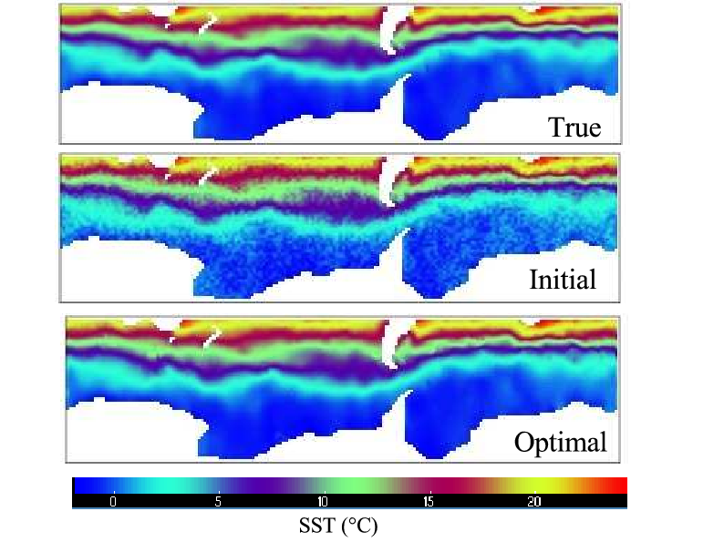
One particular case of inverse problems is data assimilation [37] in weather forecasting or in oceanography. The quality of the initial state of the simulation conditions the quality of the prediction. But this initial state is not well known. Only some measurements at arbitrary places and times are available. A good initial state is found by solving a least squares problem between the measurements and a guessed initial state which itself must verify the equations of meteorology. This boils down to solving an adjoint problem, which can be done though AD [40]. Figure 1 shows an example of a data assimilation exercise using the oceanography code OPA [38] and its AD-adjoint produced by Tapenade.
|
The special case of 4Dvar data assimilation is particularly challenging. The 4th dimension in “4D” is time, as available measurements are distributed over a given assimilation period. Therefore the least squares mechanism must be applied to a simulation over time that follows the time evolution model. This process gives a much better estimation of the initial state, because both position and time of measurements are taken into account. On the other hand, the adjoint problem involved is more complex, because it must run (backwards) over many time steps. This demanding application of AD justifies our efforts in reducing the runtime and memory costs of AD adjoint codes.