

Section: Research Program
Functional Inference, semi- and non-parametric methods
Participants : Clement Albert, Alessandro Chiancone, Stephane Girard, Seydou Nourou Sylla, Pablo Mesejo Santiago, Florence Forbes, Emeline Perthame, Jean-Michel Becu.
Key-words: dimension reduction, extreme value analysis, functional estimation.
We also consider methods which do not assume a parametric model. The approaches are non-parametric in the sense that they do not require the assumption of a prior model on the unknown quantities. This property is important since, for image applications for instance, it is very difficult to introduce sufficiently general parametric models because of the wide variety of image contents. Projection methods are then a way to decompose the unknown quantity on a set of functions (e.g. wavelets). Kernel methods which rely on smoothing the data using a set of kernels (usually probability distributions) are other examples. Relationships exist between these methods and learning techniques using Support Vector Machine (SVM) as this appears in the context of level-sets estimation (see section 3.3.2). Such non-parametric methods have become the cornerstone when dealing with functional data [77]. This is the case, for instance, when observations are curves. They enable us to model the data without a discretization step. More generally, these techniques are of great use for dimension reduction purposes (section 3.3.3). They enable reduction of the dimension of the functional or multivariate data without assumptions on the observations distribution. Semi-parametric methods refer to methods that include both parametric and non-parametric aspects. Examples include the Sliced Inverse Regression (SIR) method [80] which combines non-parametric regression techniques with parametric dimension reduction aspects. This is also the case in extreme value analysis [76], which is based on the modelling of distribution tails (see section 3.3.1). It differs from traditional statistics which focuses on the central part of distributions, i.e. on the most probable events. Extreme value theory shows that distribution tails can be modelled by both a functional part and a real parameter, the extreme value index.
Modelling extremal events
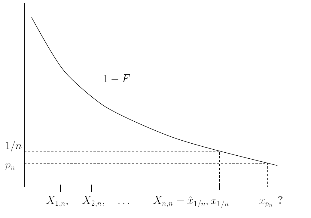
Extreme value theory is a branch of statistics dealing with the extreme deviations from the bulk of probability distributions. More specifically, it focuses on the limiting distributions for the minimum or the maximum of a large collection of random observations from the same arbitrary distribution. Let denote ordered observations from a random variable representing some quantity of interest. A -quantile of is the value such that the probability that is greater than is , i.e. . When , such a quantile is said to be extreme since it is usually greater than the maximum observation (see Figure 1).
|
To estimate such quantiles therefore requires dedicated methods to extrapolate information beyond the observed values of . Those methods are based on Extreme value theory. This kind of issue appeared in hydrology. One objective was to assess risk for highly unusual events, such as 100-year floods, starting from flows measured over 50 years. To this end, semi-parametric models of the tail are considered:
where both the extreme-value index and the function are unknown. The function is a slowly varying function i.e. such that
for all . The function acts as a nuisance parameter which yields a bias in the classical extreme-value estimators developed so far. Such models are often referred to as heavy-tail models since the probability of extreme events decreases at a polynomial rate to zero. It may be necessary to refine the model (2,3) by specifying a precise rate of convergence in (3). To this end, a second order condition is introduced involving an additional parameter . The larger is, the slower the convergence in (3) and the more difficult the estimation of extreme quantiles.
More generally, the problems that we address are part of the risk management theory. For instance, in reliability, the distributions of interest are included in a semi-parametric family whose tails are decreasing exponentially fast. These so-called Weibull-tail distributions [9] are defined by their survival distribution function:
Gaussian, gamma, exponential and Weibull distributions, among others, are included in this family. An important part of our work consists in establishing links between models (2) and (4) in order to propose new estimation methods. We also consider the case where the observations were recorded with a covariate information. In this case, the extreme-value index and the -quantile are functions of the covariate. We propose estimators of these functions by using moving window approaches, nearest neighbor methods, or kernel estimators.
Level sets estimation
Level sets estimation is a recurrent problem in statistics which is linked to outlier detection. In biology, one is interested in estimating reference curves, that is to say curves which bound (for example) of the population. Points outside this bound are considered as outliers compared to the reference population. Level sets estimation can be looked at as a conditional quantile estimation problem which benefits from a non-parametric statistical framework. In particular, boundary estimation, arising in image segmentation as well as in supervised learning, is interpreted as an extreme level set estimation problem. Level sets estimation can also be formulated as a linear programming problem. In this context, estimates are sparse since they involve only a small fraction of the dataset, called the set of support vectors.
Dimension reduction
Our work on high dimensional data requires that we face the curse of dimensionality phenomenon. Indeed, the modelling of high dimensional data requires complex models and thus the estimation of high number of parameters compared to the sample size. In this framework, dimension reduction methods aim at replacing the original variables by a small number of linear combinations with as small as a possible loss of information. Principal Component Analysis (PCA) is the most widely used method to reduce dimension in data. However, standard linear PCA can be quite inefficient on image data where even simple image distorsions can lead to highly non-linear data. Two directions are investigated. First, non-linear PCAs can be proposed, leading to semi-parametric dimension reduction methods [78]. Another field of investigation is to take into account the application goal in the dimension reduction step. One of our approaches is therefore to develop new Gaussian models of high dimensional data for parametric inference [74]. Such models can then be used in a Mixtures or Markov framework for classification purposes. Another approach consists in combining dimension reduction, regularization techniques, and regression techniques to improve the Sliced Inverse Regression method [80].