Section: Research Program

The scientific context

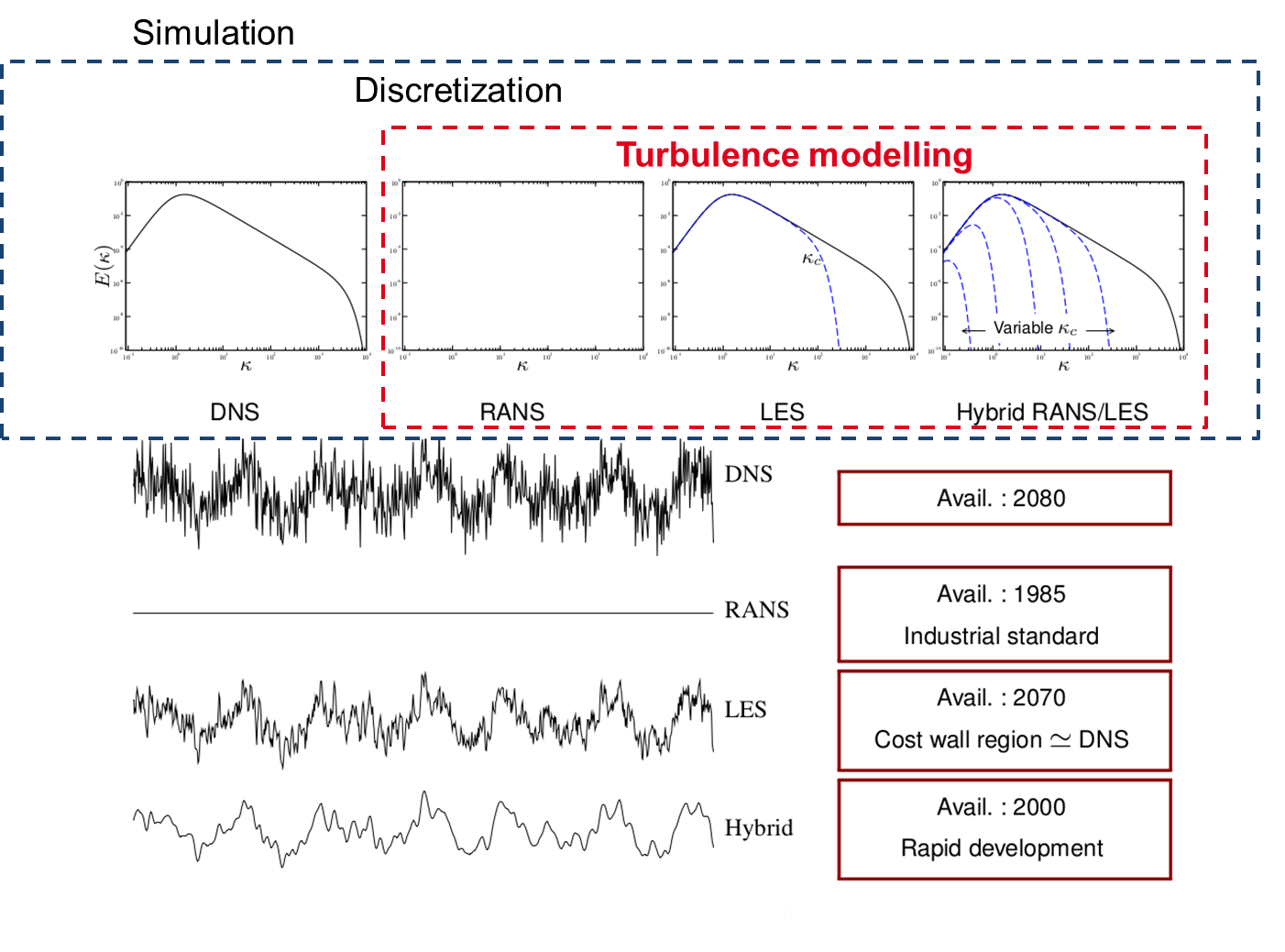
Computational fluid mechanics: modeling or not before discretizing ?

A typical continuous solution of the Navier Stokes equations at sufficiently high values of the Reynolds number is governed by a spectrum of time and space scales fluctuations closely connected with the turbulent nature of the flow. The term deterministic chaos employed by Frisch in his enlightening book [32] is certainly conveying most adequately the difficulty in analyzing and simulating this kind of flows. The broadness of the turbulence spectrum is directly controlled by the Reynolds number defined as the ratio between the inertial forces and the viscous forces. This number is not only useful to determine the transition from a laminar to a turbulent flow regime, it also indicates the range of scales of fluctuations that are present in the flow under consideration. Typically, for the velocity field and far from solid walls, the ratio between the largest scale (the integral length scale) to the smallest one (Kolmogorov scale) scales as $R{e}^{3/4}$ per dimension. In addition, for internal flows, the viscous effects near the solid walls yield a scaling proportional to $Re$ per dimension. The smallest scales play a crucial role in the dynamics of the largest ones which implies that an accurate framework for the computation of turbulent flows must take into account all these scales. Thus, the usual practice to deal with turbulent flows is to choose between an a priori modeling (in most situations) or not (low Re number and rather simple configurations) before proceeding to the discretization step followed by the simulation runs themselves. If a modeling phase is on the agenda, then one has to choose again among the above mentioned variety of approaches. As it is illustrated in Fig. 1, this can be achieved either by directly solving the Navier-Stokes equations (DNS) or by first applying a statistical averaging (RANS) or a spatial filtering operator to the Navier-Stokes equations (LES). The new terms brought about by the filtering operator have to be modeled. From a computational point of view, the RANS approach is the least demanding, which explains why historically it has been the workhorse in both the academic and the industrial sectors. It has permitted quite a substantial progress in the understanding of various phenomena such as turbulent combustion or heat transfer. Its inherent inability to provide a time-dependent information has led to promote in the last decade the recourse to either LES or DNS to supplement if not replace RANS. By simulating the large scale structures while modeling the smallest ones supposed to be more isotropic, LES proved to be quite a step through that permits to fully take advantage of the increasing power of computers to study complex flow configurations. At the same time, DNS was progressively applied to geometries of increasing complexity (channel flows with values of $R{e}_{\tau }$ multiplied by 10 during the last 15 years, jets, turbulent premixed flames, among many others), and proved to be a formidable tool that permits (i) to improve our knowledge on turbulent flows and (ii) to test (i.e., validate or invalidate) and improve the modeling hypotheses inherently associated to the RANS and LES approaches. From a numerical point of view, if the steady nature of the RANS equations allows to perform iterative convergence on finer and finer meshes, the high computational cost of LES or DNS makes necessary the use of highly accurate numerical schemes in order to optimize the use of computational resources. To the noticeable exception of the hybrid RANS-LES modeling, which is not yet accepted as a reliable tool for industrial design, as mentioned in the preamble of the Go4hybrid European program (https://cordis.europa.eu/result/rcn/177053_en.html), once chosen, a single turbulence model will (try to) do the job for modeling the whole flow. Thus, depending on its intrinsic strengths and weaknesses, the accuracy will be a rather volatile quantity strongly dependent on the flow configuration. The turbulence modeling and industrial design communities waver between the desire to continue to rely on the RANS approach, which is unrivaled in terms of computational cost, but is still not able to accurately represent all the complex phenomena; and the temptation to switch to LES, which outperforms RANS in many situations but is prohibitively expensive in high-Reynolds number wall-bounded flows. In order to account for the deficiencies of both approaches and to combine them for significantly improving the overall quality of the modeling, the hybrid RANS-LES approach has emerged during the last decade as a viable, intermediate way, and we are definitely inscribing our project in this innovative field of research, with an original approach though, connected with a time filtered hybrid RANS-LES and a systematic and progressive validation process against experimental data produced by the team.

Computational fluid mechanics: high order discretization on unstructured meshes and efficient methods of solution

All the methods considered in the project are mesh-based methods: the computational domain is divided into cells, that have an elementary shape: triangles and quadrangles in two dimensions, and tetrahedra, hexahedra, pyramids, and prisms in three dimensions. If the cells are only regular hexahedra, the mesh is said to be structured. Otherwise, it is said to be unstructured. If the mesh is composed of more than one sort of elementary shape, the mesh is said to be hybrid. In the project, the numerical strategy is based on discontinuous Galerkin methods. These methods were introduced by Reed and Hill [43] and first studied by Lesaint and Raviart [39]. The extension to the Euler system with explicit time integration was mainly led by Shu, Cockburn and their collaborators. The steps of time integration and slope limiting were similar to high order ENO schemes, whereas specific constraints given by the finite element nature of the scheme were progressively solved, for scalar conservation laws [28], [27], one dimensional systems [26], multidimensional scalar conservation laws [25], and multidimensional systems [29]. For the same system, we can also cite the work of [31], [36], which is slightly different: the stabilization is made by adding a nonlinear term, and the time integration is implicit. Contrary to continuous Galerkin methods, the discretization of diffusive operators is not straightforward. This is due to the discontinuous approximation space, which does not fit well with the space function in which the diffusive system is well posed. A first stabilization was proposed by Arnold [18]. The first application of discontinuous Galerkin methods to Navier-Stokes equations was proposed in [23] by mean of a mixed formulation. Actually, this first attempt led to a non compact computation stencil, and was later proved to be not stable. A compactness improvement was made in [24], which was later analyzed, and proved to be stable in a more unified framework [19]. The combination with the $k-\omega$ RANS model was made in [22]. As far as Navier Stokes equations are concerned, we can also cite the work of [34], in which the stabilization is closer to the one of [19], the work of [40] on local time stepping, or the first use of discontinuous Galerkin methods for direct numerical simulation of a turbulent channel flow done in [30]. Discontinuous Galerkin methods are so popular because:

• They can be developed for any order of approximation.

• The computational stencil of one given cell is limited to the cells with which it has a common face. This stencil does not depend on the order of approximation. This is a pro, compared for example with high order finite volumes, which require as more and more neighbors as the order increases.

• They can be developed for any kind of mesh, structured, unstructured, but also for aggregated grids [21]. This is a pro compared not only with finite differences schemes, which can be developed only on structured meshes, but also compared with continuous finite elements methods, for which the definition of the approximation basis is not clear on aggregated elements.

• $p$-adaptivity is easier than with continuous finite elements, because neighboring elements having a different order are only weakly coupled.

• Upwinding is as natural as for finite volumes methods, which is a benefit for hyperbolic problems.

• As the formulation is weak, boundary conditions are naturally weakly formulated. This is a benefit compared with strong formulations, for example point centered formulation when a point is at the intersection of two kinds of boundary conditions.

For concluding this section, there already exist numerical schemes based on the discontinuous Galerkin method which proved to be efficient for computing compressible viscous flows. Nevertheless, there remain many things to be improved, which include: efficient shock capturing methods for supersonic flows, high order discretization of curved boundaries, low Mach number behavior of these schemes and combination with second-moment RANS models.Another drawback of the discontinuous Galerkin methods is that they can be computationally costly, due to the accurate representation of the solution calling for a particular care of implementation for being efficient. We believe that this cost can be balanced by the strong memory locality of the method, which is an asset for porting on emerging many-core architectures.

Experimental fluid mechanics: a relevant tool for physical modeling and simulation development

With the considerable and constant development of computer performance, many people were thinking at the turn of the 21st century that in the short term, CFD would replace experiments considered as too costly and not flexible enough. Simply flipping through scientific journals such as Journal of Fluid Mechanics, Combustion of Flame, Physics of Fluids or Journal of Computational Physics or through websites such that of Ercoftac (http://www.ercoftac.org) is sufficient to convince oneself that the recourse to experiments to provide either a quantitative description of complex phenomena or reference values for the assessment of the predictive capabilities of the physical modeling and of the related simulations is still necessary. The major change that can be noted though concerns the content of the interaction between experiments and CFD (understood in the broad sense). Indeed, LES or DNS assessment calls for the experimental determination of time and space turbulent scales as well as time resolved measurements and determination of single or multi-point statistical properties of the velocity field. Thus, the team methodology incorporates from the very beginning an experimental component that is operated in strong interaction with the physical modeling and the simulation activities.