Accessibility setting

Section: New Results

Inverse problems for Poisson-Laplace equations

Participants : Paul Asensio, Laurent Baratchart, Sylvain Chevillard, Juliette Leblond, Jean-Paul Marmorat, Konstantinos Mavreas, Masimba Nemaire.

Inverse magnetization issues from planar data

The overall goal is here to determine magnetic properties of rock samples (e.g. meteorites or stalactites), from weak field measurements close to the sample that can nowadays be obtained using SQUIDs (superconducting quantum interference devices). Depending on the geometry of the rock sample, the magnetization distribution can either be considered to lie in a plane (thin sample) or in a parallelepiped of thickness $r$. Some of our results apply to both frameworks (the former appears as a limiting case when $r$ goes to 0), while others concern the 2-D case and have no 3-D counterpart as yet.

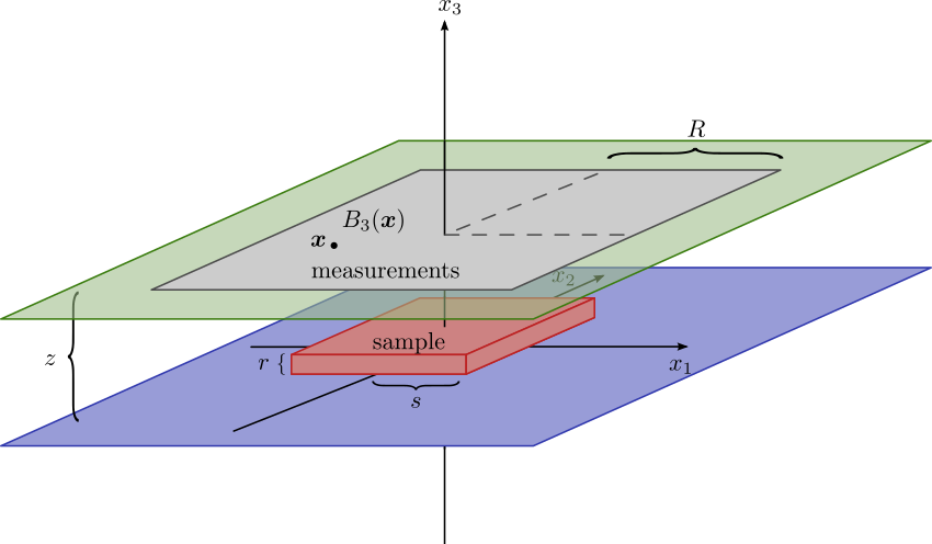
Figure 3 presents a schematic view of the experimental setup: the sample lies on a horizontal plane at height 0 and its support is included in a parallelepiped. The vertical component $B_3$ of the field produced by the sample is measured in points of a horizontal square at height $z$.

We pursued our investigation of the recovery of magnetizations modeled by signed measures on thin samples, and we singled out an interesting class that we call slender samples. These are sets of zero measure in ${ℝ}^3$, the complement of which has all its connected components of infinite measure. For such samples, we showed that consistent recovery is possible, in the Morozov discrepancy limit, by penalizing the total variation when either the support of the magnetization is purely 1-unrectifiable (which holds in particular for dipolar models) or the magnetization is unidirectional (an assumption of physical interest because igneous rocks acquire magnetization by cooling down in some ambient field). These notions play a role similar to sparsity in this infinite-dimensional context. An article has been published to report on these results [16]. Moreover, in the case of planar samples (which are certainly slender), a loop decomposition of divergence free measures was obtained, which sharpens in the 2-D setting the structure theorem of [77], and allowed us to prove, using in addition the real analyticity of the operators relating the magnetization to the field, that the argument of the minimum of the regularized criterion $\parallel f-B_3{\mu \parallel }_2^2+\lambda {\parallel \mu \parallel }_{TV}$ is unique; here, $\mu$ is the measure representing the magnetization with respect to which the criterion gets optimized, $f$ is the data and $\lambda >0$ a regularization parameter, while ${\parallel \mu \parallel }_{TV}$ is the total variation of $\mu$. An implementation using a variant of the FISTA algorithm has been set up which yields promising results when measurements are carried out on a relatively large surface patch. Yet, a deeper understanding on how to adjust the parameters of the method is required. This topic is studied in collaboration with D. Hardin and C. Villalobos from Vanderbilt University.

We also continued investigating the recovery of the moment of a magnetization, an important physical quantity which is in principle easier to reconstruct than the full magnetization because it is simply a vector in ${ℝ}^3$ that only depends on the field (i.e. magnetizations that produce the zero field also have zero moment). For the case of thin samples, we published an article reporting the construction of linear estimators for the moment from the field, based on the solution of certain bounded extremal problems in the range of the adjoint of the forward operator [15]. On a related side, we also setup other linear estimators based on asymptotic results, in the previous years. These estimators are not limited to thin samples and can in principle estimate the net moment of 3D samples, provided that the dimensions of the sample are small with respect to the measurement area. Numerical experiments confirm that linear estimators (both kinds) make essential use of field values taken at the boundary of the measurement area, and are easily blurred by noise. We experimentally confirmed this sensitivity on a rather simple case: a small spherule has been magnetized in a controlled way by our partners at MIT, and its net moment has been measured by a classical magnetometer. The spherule has then been measured with the SQUID microscope, with several choices for important parameters (height of the sensor with respect to the spherule, sensitivity of the instrument, size of the 2D rectangle on which measurements are performed, size of the sample step). We applied our (asymptotics based) linear estimator on these experimental maps and they turn out to be clearly affected, especially when the data at the edges of the map are involved. The nature of the noise due to the microscope itself (electronic and quantization noise) might play an important role, as it is known to be non-white, and therefore can affect our methods which sum it up. Subsequently, we now envisage the possibility of modeling the structure of the noise to pre-process the data.

Finally, we considered a simplified 2-D setup for magnetizations and magnetic potentials (of which the magnetic field is the gradient). When both the sample and the measurement set are parallel intervals, we set up some best approximation issues related to inverse recovery and relevant BEP problems in Hardy classes of holomorphic functions, see Section 3.3.1 and [25], which is joint work with E. Pozzi (Department of Mathematics and Statistics, St Louis Univ., St Louis, Missouri, USA). Note that, in the present case, the criterion no longer acts on the boundary of the holomorphy domain (namely, the upper half-plane), but on a strict subset thereof, while the constraint acts on the support of the approximating function. Both involve functions in the Hilbert Hardy space of the upper half-plane.

Inverse magnetization issues from sparse cylindrical data

The team Factas was a partner of the ANR project MagLune on Lunar magnetism, headed by the Geophysics and Planetology Department of Cerege, CNRS, Aix-en-Provence, which ended this year (see Section 8.2.1). Recent studies let geoscientists think that the Moon used to have a magnetic dynamo for a while. However, the exact process that triggered and fed this dynamo is still not understood, much less why it stopped. The overall goal of the project was to devise models to explain how this dynamo phenomenon was possible on the Moon.

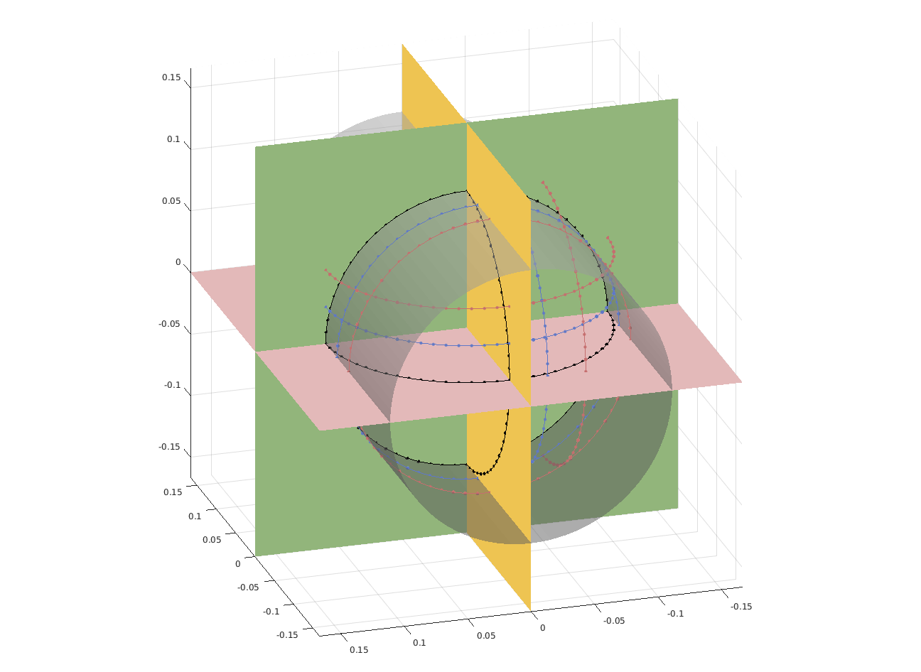
The geophysicists from Cerege went a couple of times to NASA to perform measurements on a few hundreds of samples brought back from the Moon by Apollo missions. The samples are kept inside bags with a protective atmosphere, and geophysicists are not allowed to open the bags, nor to take out samples from NASA facilities. Moreover, the process must be carried out efficiently as a fee is due to NASA by the time when handling these moon samples. Therefore, measurements were performed with some specific magnetometer designed by our colleagues from Cerege. This device measures the components of the magnetic field produced by the sample, at some discrete set of points located on circles belonging to three cylinders (see Figure 4). The objective of Factas is to enhance the numerical efficiency of post-processing data obtained with this magnetometer.

Under the hypothesis that the field can be well explained by a single magnetic pointwise dipole, and using ideas similar to those underlying the FindSources3D tool (see Sections 3.4.3 and 6.1.3), we try to recover the position and the moment of the dipole using the available measurements. This work, which is still on-going, constitutes the topic of the PhD thesis of K. Mavreas, whose defense is scheduled on January 31, 2020. In a given cylinder, using the associated cylindrical system of coordinates, recovering the position of the dipole boils down to determine its height $z$, its radial distance $\rho$ and its azimuth $\phi$. We use the fact that, whatever component of the field is measured, the (square of the) measurements performed on the circle at height $h$ correspond to a rational function of the form $p\left(z\right)/{(z-u_h)}^5$ where $p$ is a polynomial of degree at most 4 and $u_h$ is the complex number $u_h=\frac{1+{\rho }^2+{(h-z)}^2}{\rho }{e}^{i\phi }$. The numerator $p$ depends on the moment of the dipole, on the height $h$ and on the kind of component which is measured. In contrast, $u_h$ can be estimated by rational approximation techniques, which allows one to obtain $\phi$ directly and gives the relation $\rho |u_h|=1+{\rho }^2+{(h-z)}^2$. Combining the relations obtained at several heights, we proposed several methods to estimate $\rho$ and $z$.

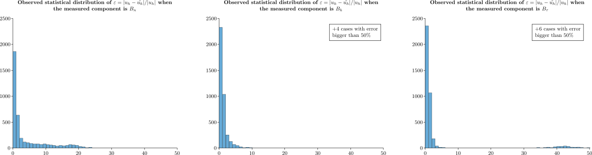
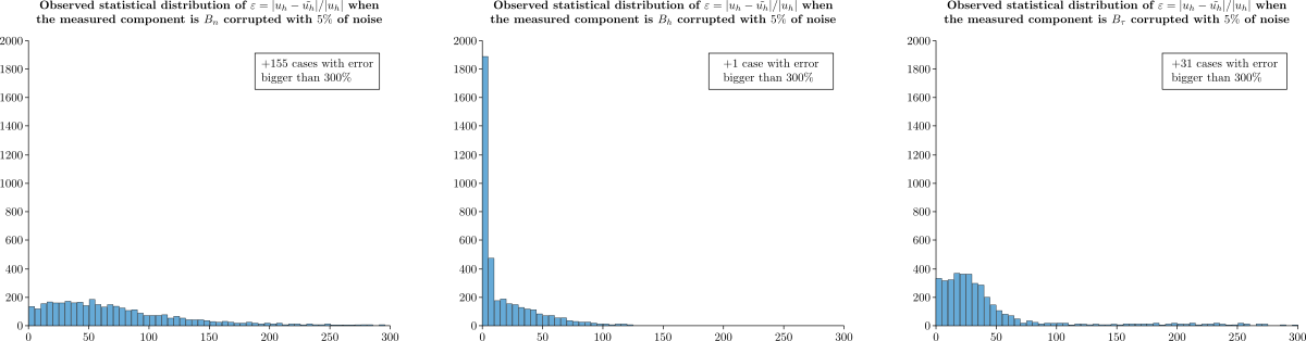
This year has been mostly devoted to running numerical experiments on synthetic examples. The first important observation is that the minimization criterion that we use to recover $u_h$ can have local minima achieving very small values, and that can sometimes erroneously be considered as the global minimum. We started studying theoretically this phenomenon, see Section 6.7.1. This means that the relative error $\epsilon =|u_h-\widetilde{u_h}|/|u_h|$ between the theoretical minimum $u_h$ and the value $\widetilde{u_h}$ estimated by our algorithm can vary from almost 0 to more than $50\%$, even when the data used as measurements exactly correspond to the field produced by a magnetic dipole. The second important observation is that the statistical distribution of $\epsilon$ (when the position of the dipole is uniformly chosen within a cylinder with a moment uniformly chosen on the unit sphere) depends on the measured component of the field. Figure 5 shows the distribution experimentally observed. The vertical component of the field noticeably leads to better estimates for $u_h$ than both other components. The third important observation that we made is that the presence of noise on the measurements, even moderate, significantly alters the quality of the estimation of $u_h$. Figure 6 shows the distribution experimentally observed in the same conditions as before, but using data contaminated with a random normal noise with standard deviation $5\%$ of the maximal absolute value of the measured component.

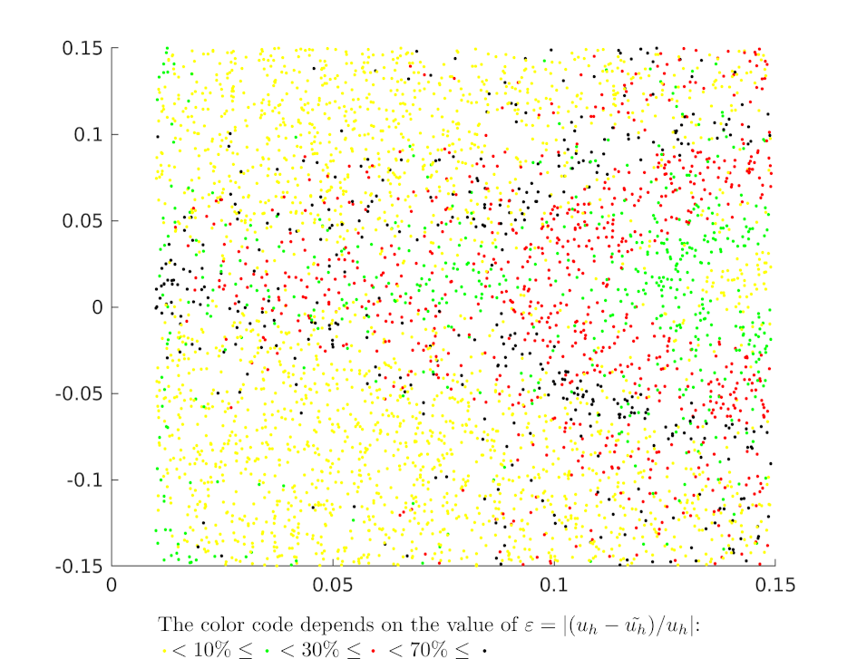
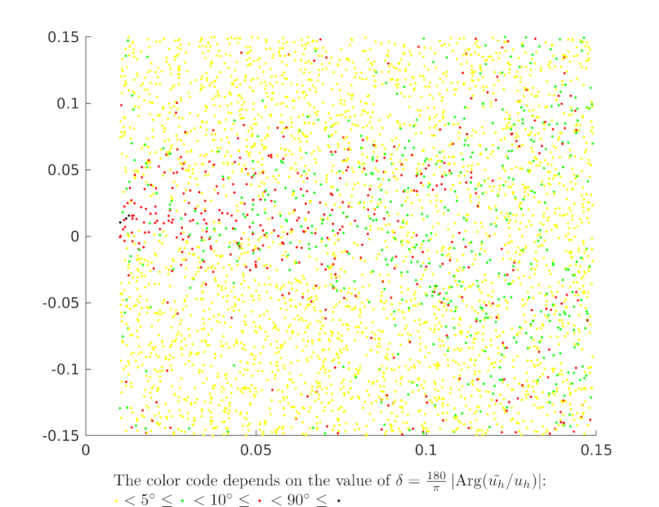
These observations are somehow bad news, as the method we propose is based on recovering the position of the dipole by using the values $u_h$ collected at several heights $h$. However, our experiments also revealed an unexpected good news: while the estimation of $u_h$ itself is often bad, as soon as the data are not perfect, its argument (from which $\phi$ is immediately deduced) turns out to be fairly well recovered. This is illustrated in Figure 7 which shows, on the set of experiments of Figure 6, the position of the 4000 dipoles, with a color indicating whether $\epsilon$ is big (left part of the figure) and whether the error on the argument of $u_h$ is big (right part of the figure). As can be seen, the angular error is most of the time smaller than $10°$, even for dipoles for which $\epsilon$ is fairly big. This phenomenon is probably due to the fact that local minima of the criterion tends to have a complex argument close to the complex argument of the global minimum, a phenomenon that we started to study theoretically (see Section 6.7.1).

Inverse problems in medical imaging

In 3-D, functional or clinically active regions in the cortex are often modeled by pointwise sources that have to be localized from measurements, taken by electrodes on the scalp, of an electrical potential satisfying a Laplace equation (EEG, electroencephalography). In the works [8], [42] on the behavior of poles in best rational approximants of fixed degree to functions with branch points, it was shown how to proceed via best rational approximation on a sequence of 2-D disks cut along the inner sphere, for the case where there are finitely many sources (see Section 4.3).

In this connection, a dedicated software FindSources3D (FS3D, see Section 3.4.3) is being developed, in collaboration with the Inria team Athena and the CMA - Mines ParisTech. Its Matlab version now incorporates the treatment of MEG data, the aim being to handle simultaneous EEG–MEG recordings available from our partners at INS, hospital la Timone, Marseille. Indeed, it is now possible to use simultaneously EEG and MEG measurement devices, in order to measure both the electrical potential and a component of the magnetic field (its normal component on the MEG helmet, that can be assumed to be spherical). This enhances the accuracy of our source recovery algorithms. Note that FS3D takes as inputs actual EEG measurements, like time signals, and performs a suitable singular value decomposition in order to separate independent sources.

It appears that, in the rational approximation step, multiple poles possess a nice behavior with respect to branched singularities. This is due to the very physical assumptions on the model from dipolar current sources: for EEG data that correspond to measurements of the electrical potential, one should consider triple poles; this will also be the case for MEG – magneto-encephalography – data. However, for (magnetic) field data produced by magnetic dipolar sources, like in Section 6.1.2, one should consider poles of order five. Though numerically observed in [9], there is no mathematical justification so far why multiple poles generate such strong accumulation of the poles of the approximants (see Section 6.7.1). This intriguing property, however, is definitely helping source recovery and will be the topic of further study. It is used in order to automatically estimate the “most plausible” number of sources (numerically: up to 3, at the moment).

This year, we started considering a different class of models, not necessarily dipolar, and related estimation algorithms. Such models may be supported on the surface of the cortex or in the volume of the encephalon. We represent sources by vector-valued measures, and in order to favor sparsity in this infinite-dimensional setting we use a TV (i.e. total variation) regularization term as in Section 6.1.1. The approach follows that of [16] and is implemented through two different algorithms, whose convergence properties are currently being studied. Tests on synthetic data from a few dipolar sources provide results of different qualities that need to be better understood. In particular, a weight is being added in the TV term in order to better identify deep sources. This is the topic of the starting PhD research of P. Asensio and M. Nemaire. Ultimately, the results will be compared to those of FS3D and other available software tools.