

Section: Research Program
Thermal methods
Infrared vision and measurement Method
This section introduce the infrared radiation and its link with the temperature, in the next part different measurement methods based on that principle are presented.
Infrared radiation
Infrared is an electromagnetic radiation having a wavelength between and 1 , this range begin early after the visible spectrum and it ends on the microwaves domain, see Figure 1 .
|
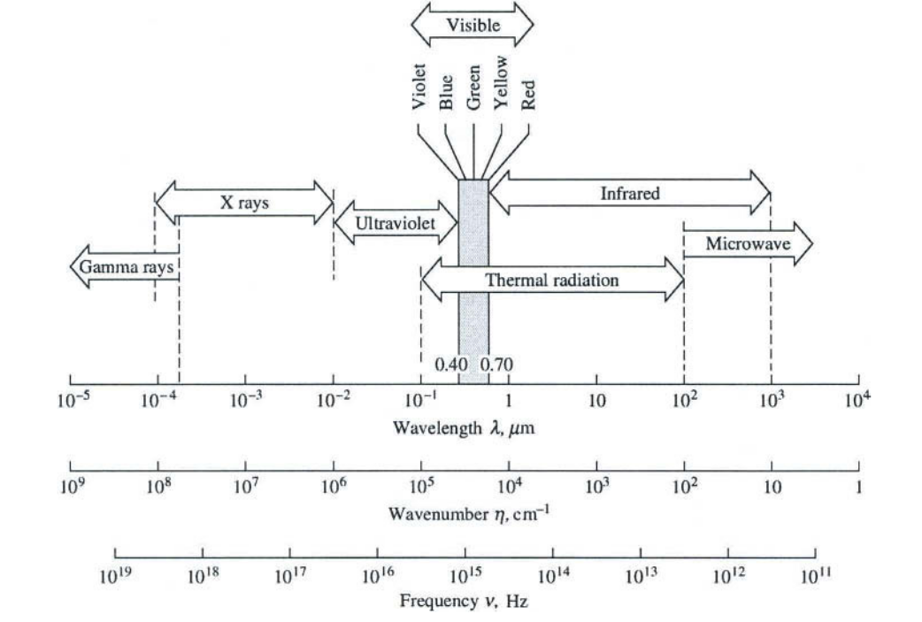
For scientific purpose infrared can be divided in three ranges of wavelength in which the application varies, see Table 1 .
| Band name | wavelength | Uses definition |
| Near infrared (PIR, IR-A, NIR) | m | Reflected solar heat flux |
| Mid infrared (MIR, IR-B) | m | Thermal infrared |
| Far infrared (LIR, IR-C, FIR) | m | Astronomy |
Our work is concentrated in the mid infrared spectral band. Keep in mind that Table 1 represents the ISO 20473 division scheme, in the literature boundaries between bands can move slightly.
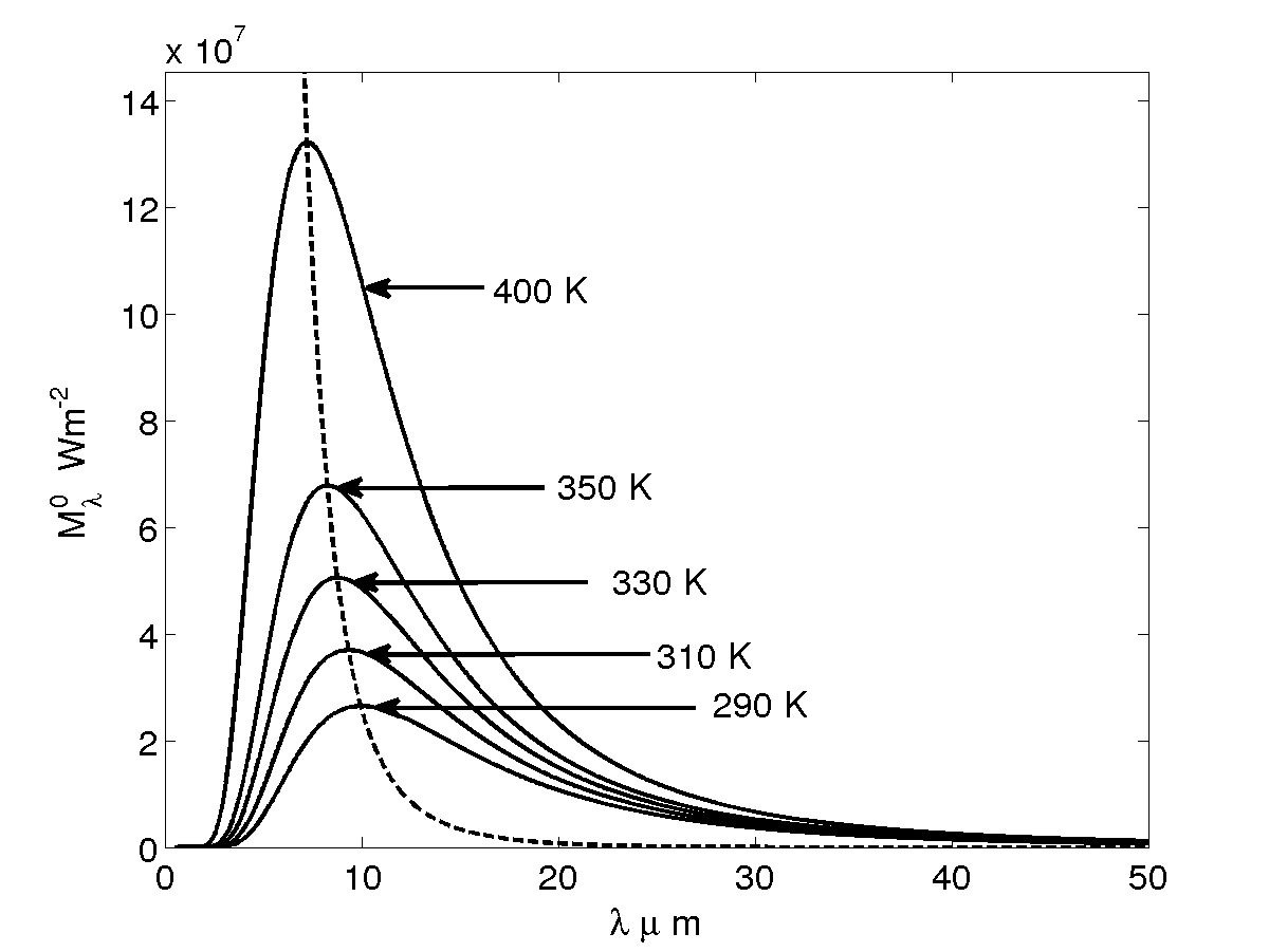
The Plank's law, proposed by Max Planck en 1901, allow to compute the black body emission spectrum for various temperatures (and only temperatures), see Figure 2 left. The black body is a theoretical construction, it represents perfect energy transmitter at a given temperature, cf Equation (20 ).
With the wavelength in m and as the temperature in Kelvin. The an constant, respectively in kg.m.s and m.K are defined as follow:
with
-
The electromagnetic wave speed (in vacuum is the light speed in m.s).
-
J.K The Boltzmann (Entropy definition from Ludwig Boltzmann 1873). It can be seen as a proportionality factor between the temperature and the energy of a system.
-
J.s The Plank constant. It's the link between the photons energy and their frequency.
By generalizing the Plank's law with the Stefan Boltzmann law ( proposed first in 1879 and then in 1884 by Joseph Stefan and Ludwig Boltzmann) it's possible to address mathematically the energy spectrum of real body at each wavelength dependent of the temperature, the optical condition and the real body properties, which is the base of the infrared thermography, cf Equation (22 ).
where
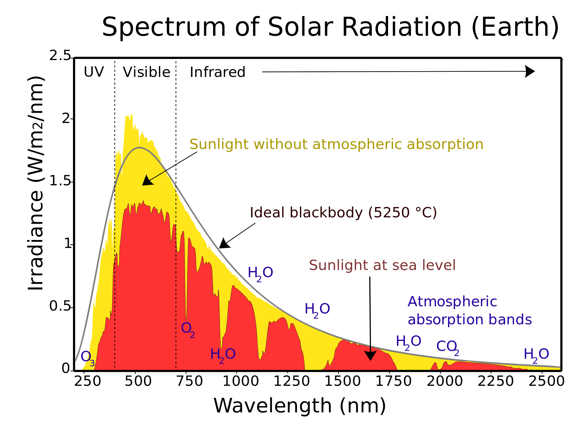
For example, Figure 2 right presents the energy spectrum of the atmosphere at various levels, it can be seen that the various properties of the atmosphere affect the spectrum at various wavelengths. Other important point is that the infrared solar heat flux can be approximated by a black body at 5523,15 K.
The above demonstrations are here to illustrate how energy and temperature can be linked, this can only be used as an general purpose introduction for the next sections.
Infrared Thermography
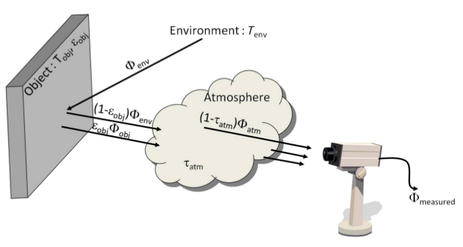
The infrared thermography is a way to measure the thermal radiation emitted or reflected by a medium. With that information about the electromagnetic flux it's possible to compute the surface temperature of the body, see section 3.2.1.1 . Various types of detector can assure the measure of the electromagnetic radiation. Table 2 illustrates for various spectral bands in infrared some of the detectors which can be used to measure the thermal radiation.
| Bands | Wavelength | Detectors |
| Near Infrared | End of the human eye response, Aluminium gallium arsenide detectors (InGaAs) | |
| Short Wave Infrared - SWIR\Band I | Germanium detector ans InGaAs | |
| Mid Wave Infrared - MWIR\Band II | Mercury cadmium telluride detectors (HgCdTe), Lead selenide (PbSe) and InSb | |
| Long wave Infrared - LWIR\Band III | Microbolometers (VOx) and HgCdTe | |
| Very long wave infrared | silicon detectors |
|
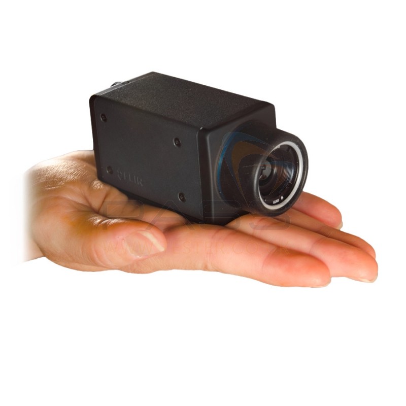
Those different detectors can take various forms and/or manufacturing process. For our research purpose we use uncooled infrared camera using a matrix of microbolometers detectors. A microbolometer, as a lot of transducers, converts a radiation in electric current used to represent the physical quantity (here the heat flux). Figure 3 shows an example of FLIR AX5 low cost mini infrared camera that we use for long term SHM purpose, and also a schematic representation of the measurement principle.
This field of activity includes the use and the improvement of vision system, like in [6] .
Heat transfer theory
Once the acquisition process is done, it's useful to model the heat conduction inside the cartesian domain . Note that in opaque solid medium the heat conduction is the only mode of heat transfer. Proposed by Jean Baptiste Biot in 1804 and experimentally demonstrated by Joseph Fourier in 1821, the Fourier Law describes the heat flux inside a solid, cf Equation (23 ).
Where is the thermal conductivity in W.m.K , is the gradient operator and is the heat flux density in Wm. This law illustrates the first principle of thermodynamic (law of conservation of energy) and implies the second principle (irreversibility of the phenomenon), from this law it can be seen that the heat flux always goes from hot area to cold area.
An energy balance with respect to the first principle drives to the expression of the heat conduction in all point of the domain , cf Equation (24 ). This equation has been proposed by Joseph Fourier in 1811.
With the divergence operator, the specific heat capacity in J.kg.K, the volumetric mass density in kg. m, the space variable and a possible internal heat production in W.m.
To solve the system (24 ), it's necessary to express the boundaries conditions of the system. With the developments presented in section 3.2.1.1 and the Fourier's law it's possible, for example, to express the thermal radiation and the convection phenomenon which can occur at the system boundaries, cf Equation (25 ).
Equation (25 ) is the so called Robin condition on the boundary , where is the normal, the convective heat transfer coefficient in W.m.K and an external energy contribution W.m, in cases where the external energy contribution is artificial and controlled we call it active thermography (spotlight etc...) in the contrary it's called passive thermography (direct solar heat flux).
The systems presented in the different sections above ( 3.2.1 to 3.2.2 ) are useful to build physical models in order to represents the measured quantity. To estimate key parameters, as the conductivity, one way to do is the model inversion, the next section will introduce that principle.
Inverse model for parameters estimation
Lets take any model which can for example represent the conductive heat transfer in a medium, the model is solved for a parameter vector and it results another vector , cf Equation (26 ). For example if represents the heat transfer, can be the temperature evolution.
With a matrix of size , a vector of size and of size , preferentially . This model is called direct model, the inverse model consist to find a vector which satisfy the results of the direct model. For that we need to inverse the matrix , cf Equation (27 ).
Here we want find the solution which is closest to the acquired measures , Equation (28 ).
To do that it's important to respect the well posed condition established by Jacques Hadamard in 1902
Unfortunately those condition are rarely respected in our field of study. That's why we dont solve directly the system (28 ) but we minimise the quadratic coast function (29 ) which represents the Legendre-Gauss least square algorithm for linear problems.
Where can be a product of matrix.
In some case the problem is still ill-posed and need to be regularized for example using the Tikhonov regularization. An elegant way to minimize the cost function is compute the gradient, Equation (31 ) and find where it's equal to zero..
Where is the sensitivity matrix of the model to its parameter vector .
Until now the inverse method proposed is valid only when the model is linearly dependent of its parameter , for the heat equation it's the case when you want to estimate the external heat flux, in equation 25 . For all the other parameters, like the conductivity the model is non-linearly dependant of its parameter . For such case the use of iterative algorithm is needed, for example the Levenberg-Marquardt algorithm, cf Equation (32 ).
Equation (32 ) is solved iteratively at each loop . Some of our results with such linear or non linear method can be seen in [7] or [2] , more specifically [1] is a custom implementation of the Levenberg-Marquardt algorithm based on the adjoin method (developed by Jacques Louis Lions in 1968) coupled to the conjugate gradient algorithm to estimate wide properties field in a medium.