

Section: Research Program
Reflectometry-based methods for electrical engineering and for civil engineering
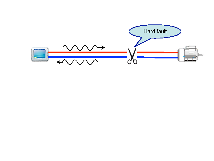
The fast development of electronic devices in modern engineering systems involves more and more connections through cables, and consequently, with an increasing number connexion failures. Wires and connectors are subject to aging and degradation, sometimes under severe environmental conditions. In many applications, the reliability of electrical connexions is related to the quality of production or service, whereas in critical applications reliability becomes also a safety issue. It is thus important to design smart diagnosis systems able to detect connection defects in real time. This fact has motivated research projects on methods for fault diagnosis in this field. Some of these projects are based on techniques of reflectometry, which consist in injecting waves into a cable or a network and in analyzing the reflections, as in the example of cable hard fault diagnosis illustrated in Figure 4 . Depending on the injected waveforms and on the methods of analysis, various techniques of reflectometry are available. They all have the common advantage of being non destructive.
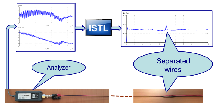
At Inria the research activities on reflectometry started within the SISYPHE EPI several years ago and now continue in the I4S EPI. Our most notable contribution in this area is a method based on the inverse scattering theory for the computation of distributed characteristic impedance along a cable from reflectometry measurements [14] , [11] , [52] . It provides an efficient solution for the diagnosis of soft faults in electrical cables, like in the example illustrated in Figure 5 . While most reflectometry methods for fault diagnosis are based on the detection and location of impedance discontinuity, our method yielding the spatial profile of the characteristic impedance is particularly suitable for the diagnosis of soft faults with no or weak impedance discontinuities.
Fault diagnosis for wired networks have also been studied in Inria [54] , [50] . The main results concern, on the one hand, simple star-shaped networks from measurements made at a single node, on the other hand, complex networks of arbitrary topological structure with complete node observations.
Though initially our studies on reflectometry were aiming at applications in electrical engineering, through our collaboration with IFSTTAR, we are also investigating applications in the field of civil engineering, by using electrical cables as sensors for monitoring changes in mechanical structures.
What follows is about some basic elements on mathematical equations of electric cables and networks, the main approach we follow in our study, and our future research directions.
Mathematical model of electric cables and networks
A cable excited by a signal generator can be characterized by the telegrapher's equations [51]
where represents the time, is the longitudinal coordinate along the cable, and are respectively the voltage and the current in the cable at the time instant and at the position , and denote respectively the series resistance, the inductance, the capacitance and the shunt conductance per unit length of the cable at the position . The left end of the cable (corresponding to ) is connected to a voltage source with internal impedance . The quantities , , and are related by
At the right end of the cable (corresponding to ), the cable is connected to a load of impedance , such that
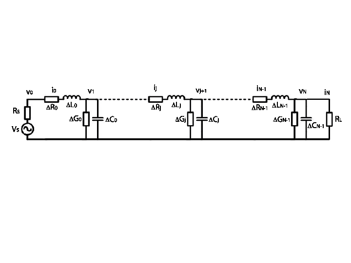
One way for deriving the above model is to spatially discretize the cable and to characterize each small segment with 4 basic lumped parameter elements, as illustrated in Figure 6 for the -th segment: a resistance , an inductance , a capacitance and a conductance . The entire circuit is described by a system of ordinary differential equations. When the spatial discretization step size tends to zero, the limiting model leads to the telegrapher's equations (33 ).
A wired network is a set of cables connected at some nodes, where loads and sources can also be connected. Within each cable the current and voltage satisfy the telegrapher's equations (33 ), whereas at each node the current and voltage satisfy the Kirchhoff's laws, unless in case of connector failures. .
The inverse scattering theory applied to cables
The inverse scattering transform was developed during the 1970s-1980s for the analysis of some nonlinear partial differential equations [49] . The visionary idea of applying this theory to solving the cable inverse problem goes also back to the 1980s [48] . After having completed some theoretic results directly linked to practice [14] , [52] , we started to successfully apply the inverse scattering theory to cable soft fault diagnosis, in collaboration with GEEPS-SUPELEC [16] .
To link electric cables to the inverse scattering theory, the telegrapher's equations (33 ) are transformed in a few steps to fit into a particular form studied in the inverse scattering theory. The Fourier transform is first applied to transform the time domain model (33 ) into the frequency domain, the spatial coordinate is then replaced by the propagation time
and the frequency domain variables are replaced by the pair
with
These transformations lead to the Zakharov-Shabat equations
with
These equations have been well studied in the inverse scattering theory, for the purpose of determining partly the “potential functions” and from the scattering data matrix, which turns out to correspond to the data typically collected with reflectometry instruments. For instance, it is possible to compute the function defined in (37 ), often known as the characteristic impedance, from the reflection coefficient measured at one end of the cable. Such an example is illustrated in Figure 5 . Any fault affecting the characteristic impedance, like in the example of Figure 5 caused by a slight geometric deformation, can thus be efficiently detected, located and characterized.