Section: Scientific Foundations

Fast parametric estimation and its applications

Parametric estimation may often be formalized as follows:

where:

• the measured signal $y$ is a functional $F$ of the "true" signal $x$, which depends on a set $\Theta$ of parameters,

• $n$ is a noise corrupting the observation.

Finding a "good" approximation of the components of $\Theta$ has been the subject of a huge literature in various fields of applied mathematics. Most of those researches have been done in a probabilistic setting, which necessitates a good knowledge of the statistical properties of $n$. Our project is devoted to a new standpoint which does not require this knowledge and which is based on the following tools, which are of algebraic flavor:

• differential algebra(Differential algebra was introduced in nonlinear control theory by one of us almost twenty years ago for understanding some specific questions like input-output inversion. It allowed to recast the whole of nonlinear control into a more realistic light. The best example is of course the discovery of flat systems which are now quite popular in industry.), which plays with respect to differential equations a similar role to commutative algebra with respect to algebraic equations;

• module theory, i.e., linear algebra over rings which are not necessarily commutative;

• operational calculus which was the most classical tool among control and mechanical engineers(Operational calculus is often formalized via the Laplace transform whereas the Fourier transform is today the cornerstone in estimation. Note that the one-sided Laplace transform is causal, but the Fourier transform over $R$ is not.).

Linear identifiability

In most problems appearing in linear control as well as in signal processing, the unknown parameters are linearly identifiable: standard elimination procedures are yielding the following matrix equation

where:

• ${\theta }_i$, $1\le i\le r$, represents unknown parameter,

• $P$ is a $r\times r$ square matrix and $Q$ is a $r\times 1$ column matrix,

• the entries of $P$ and $Q$ are finite linear combinations of terms of the form $t^{\nu }\frac{d^{\mu }\xi }{d{t}^{\mu }}$, $\mu ,\nu \ge 0$, where $\xi$ is an input or output signal,

• the matrix $P$ is generically invertible, i.e.,  $det\left(P\right)\ne 0$.

How to deal with perturbations and noises?

With noisy measurements equation (2 ) becomes:

where $R$ is a $r\times 1$ column matrix, whose entries are finite linear combination of terms of the form $t^{\nu }\frac{d^{\mu }\eta }{d{t}^{\mu }},\mu ,\nu \ge 0$, where $\eta$ is a perturbation or a noise.

Structured perturbations

A perturbation $\pi$ is said to be structured if, and only if, it is annihilated by a linear differential operator of the form ${\sum }_{\text{finite}}{a}_k\left(t\right)\frac{d^k}{d{t}^k}$, where $a_k\left(t\right)$ is a rational function of $t$, i.e.,  $\left({\sum }_{\text{finite}}{a}_k\left(t\right)\frac{d^k}{d{t}^k}\right)\pi =0$. Note that many classical perturbations like a constant bias are annihilated by such an operator. An unstructured noise cannot be annihilated by a non-zero differential operator.

By well known properties of the non-commutative ring of differential operators, we can multiply both sides of equation (3 ) by a suitable differential operator $\Delta$ such that equation (3 ) becomes:

where the entries of the $r\times 1$ column matrix $R^{\text{'}}$ are unstructured noises.

Attenuating unstructured noises

Unstructured noises are usually dealt with stochastic processes like white Gaussian noises. They are considered here as highly fluctuating phenomena, which may therefore be attenuated via low pass filters. Note that no precise knowledge of the statistical properties of the noises is required.

Comments

Although the previous noise attenuation(It is reminiscent to what most practitioners in electronics are doing.) may be fully explained via formula (4 ), its theoretical comparison(Let us stress again that many computer simulations and several laboratory experiments have been already successfully achieved and can be quite favorably compared with the existing techniques.) with today's literature(Especially in signal processing.) has yet to be done. It will require a complete resetting of the notions of noises and perturbations. Besides some connections with physics, it might lead to quite new "epistemological" issues  [80] .

Some hints on the calculations

The time derivatives of the input and output signals appearing in equations (2 ), (3 ), (4 ) can be suppressed in the two following ways which might be combined:

• integrate both sides of the equation a sufficient number of times,

• take the convolution product of both sides by a suitable low pass filter.

The numerical values of the unknown parameters $\Theta =({\theta }_1,\cdots ,{\theta }_r)$ can be obtained by integrating both sides of the modified equation (4 ) during a very short time interval.

A first, very simple example

Let us illustrate on a very basic example, the grounding ideas of the algebraic approach, based on algebra. For this, consider the first order, linear system:

where $a$ is an unknown parameter to be identified and ${\gamma }_0$ is an unknown, constant perturbation. With the notations of operational calculus and $y_0=y\left(0\right)$, equation (5 ) reads:

where $\widehat{y}\left(s\right)$ represents Laplace transform.

In order to eliminate the term ${\gamma }_0$, multiply first the two hand-sides of this equation by $s$ and, then, take their derivatives with respect to $s$:

Recall that ${\widehat{y}}^{\text{'}}\left(s\right)\triangleq \frac{d\widehat{y}\left(s\right)}{ds}$ corresponds to $-ty\left(t\right)$. Assume $y_0=0$ for simplicity's sake(If $y_0\ne 0$ one has to take above derivatives of order 2 with respect to $s$, in order to eliminate the initial condition.). Then, for any $\nu >0$,

For $\nu =3$, we obtained the estimated value $a$:

Since $T>0$ can be very small, estimation via (10 ) is very fast.

Note that equation (10 ) represents an on-line algorithm that only involves two kinds of operations on $u$ and $y:$ (1) multiplications by $t$, and (2) integrations over a pre-selected time interval.

If we now consider an additional noise, of zero mean, in (5 ), say:

it will be considered as fast fluctuating signal. The order $\nu$ in (9 ) determines the order of iterations in the integrals (3 integrals in (10 )). Those iterated integrals are low-pass filters which are attenuating the fluctuations.

This example, even simple, clearly demonstrates how algebraic's techniques proceed:

• they are algebraic: operations on $s$-functions;

• they are non-asymptotic: parameter $a$ is obtained from (10 ) in finite time;

• they are deterministic: no knowledge of the statistical properties of the noise $n$ is required.

A second simple example, with delay

Consider the first order, linear system with constant input delay(This example is taken from  [69] . For further details, we suggest the reader to refer to it.):

Here we use a distributional-like notation where $\delta$ denotes the Dirac impulse and $H$ is its integral, i.e., the Heaviside function (unit step)(In this document, for the sake of simplicity, we make an abuse of the language since we merge in a single notation the Heaviside function $H$ and the integration operator. To be rigorous, the iterated integration ($k$ times) corresponds, in the operational domain, to a division by $s^k$, whereas the convolution with $H$ ($k$ times) corresponds to a division by $s^k/(k-1)!$. For $k=0$, there is no difference and $H*y$ realizes the integration of $y$. More generally, since we will always apply these operations to complete equations (left- and right-hand sides), the factor $(k-1)!$ makes no difference.). Still for simplicity, we suppose that the parameter $a$ is known. The parameter to be identified is now the delay $\tau$. As previously, ${\gamma }_0$ is a constant perturbation, $a$, $b$, and $\tau$ are constant parameters. Consider also a step input $u=u_{0}H$. A first order derivation yields:

where ${\delta }_{\tau }$ denotes the delayed Dirac impulse and ${\varphi }_0=(\dot{y}\left(0\right)+ay\left(0\right))\delta +y\left(0\right){\delta }^{\left(1\right)}$, of order 1 and support $\left\{0\right\}$, contains the contributions of the initial conditions. According to Schwartz theorem, multiplication by a function $\alpha$ such that $\alpha \left(0\right)={\alpha }^{\text{'}}\left(0\right)=0$, $\alpha \left(\tau \right)=0$ yields interesting simplifications. For instance, choosing $\alpha \left(t\right)=t^3-\tau t^2$ leads to the following equalities (to be understood in the distributional framework):

The delay $\tau$ becomes available from $k\ge 1$ successive integrations (represented by the operator $H$), as follows:

where the $w_i$ are defined, using the notation $z_i=t^{i}y$, by:

These coefficients show that $k\ge 2$ integrations are avoiding any derivation in the delay identification.

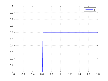
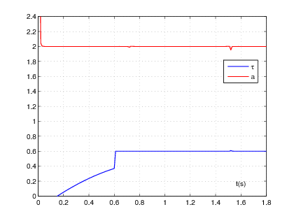
Figure 1 gives a numerical simulation with $k=2$ integrations and $a=2,b=1,\tau =0.6$, $y\left(0\right)=0.3,{\gamma }_0=2,u_0=1$. Due to the non identifiability over $(0,\tau )$, the delay $\tau$ is set to zero until the numerator or the denominator in the right hand side of (15 ) reaches a significant nonzero value.

Again, note the realization algorithm (15 ) involves two kinds of operators: (1) integrations and (2) multiplications by $t$.

It relies on the measurement of $y$ and on the knowledge of $a$. If $a$ is also unknown, the same approach can be utilized for a simultaneous identification of $a$ and $\tau$. The following relation is derived from (14 ):

and a linear system with unknown parameters $(\tau ,a\tau ,a)$ is obtained by using different integration orders:

The resulting numerical simulations are shown in Figure 2 . For identifiability reasons, the obtained linear system may be not consistent for $t<\tau$.